Root finding with scipy.optimize: Halley's comet from Kepler's equation

The problem: where is Halley's comet on a given day?

Halley's comet runs on an ellipse of eccentricity \(e = 0.967\) with a period of 75.3 years, in JPL's orbital elements for the epoch 17 February 1994, and it next passes the Sun on 28 July 2061. On 1 January 2061, 208 days earlier, a two-body model puts it 3.28 AU from the Sun, but no formula hands you that number. The date fixes the mean anomaly \(M\), the position needs the eccentric anomaly \(E\), and Kepler's equation ties them,

\[E - e\sin E = M ,\]

which no algebra solves for \(E\). Finding \(E\) is root finding, the search for the zero of \(f(E) = E - e\sin E - M\), and scipy.optimize has the tools for it.

Both angles live on the auxiliary circle of radius \(a\), the semi-major axis, drawn around the center of the ellipse. Slide the comet perpendicular to the major axis onto that circle: the angle of that point, seen from the center, is \(E\). \(M\) is the angle of a point that runs around the same circle at constant speed with the comet's period. By Kepler's second law the area swept since perihelion grows at a constant rate, so it is \(\tfrac{ab}{2}M\), with \(b\) the semi-minor axis. Written in \(E\), the same area is \(\tfrac{ab}{2}(E - e\sin E)\), and setting the two equal is Kepler's equation. In the true anomaly \(\nu\) of your orbit equation, the swept area has no form you could invert.

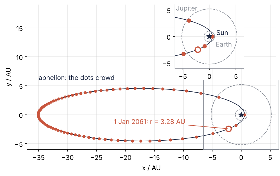
Orbit of Halley's comet in its plane, x and y in AU, Sun at the origin, one dot per year after perihelion. The dots crowd at aphelion near x = -35 AU. An inset on the inner 6 AU shows only three inside Jupiter's orbit and the comet 3.28 AU from the Sun on 1 January 2061.

The dots are the comet once a year after perihelion, all 76 from one call to newton: they crowd at the far end and rush past the Sun. The model has two bodies. The planets shift each return by months to a year or more, so the orbit is counted from the nearest perihelion.

Setup

The two orbital elements are all the data. Kepler's third law in solar units gives the semi-major axis in AU from the period in years.

import warnings
import numpy as np
import matplotlib.pyplot as plt
from scipy.optimize import brentq, newton, root_scalar

plt.rcParams.update({
    "figure.figsize": (7, 3.6), "figure.dpi": 110,
    "axes.spines.top": False, "axes.spines.right": False,
    "axes.grid": True, "grid.alpha": 0.25,
    "font.size": 11, "lines.linewidth": 1.8,
})
INK, ACCENT, SECOND, MUTED = "#1f2a44", "#c8553d", "#2a7f9e", "#8a8f98"

e = 0.967                   # eccentricity of 1P/Halley, JPL elements at epoch 1994-02-17
P = 75.3                    # orbital period / yr, same epoch
a = P ** (2 / 3)            # semi-major axis / AU, Kepler's third law
b = a * np.sqrt(1 - e**2)   # semi-minor axis / AU

def mean_anomaly(t_years):
    # wrapped to [0, 2π): the bracket [0, 2π] of Step 2 holds only there (Pitfalls)
    return np.mod(2 * np.pi * np.asarray(t_years) / P, 2 * np.pi)

print(f"a = {a:.2f} AU   perihelion {a * (1 - e):.2f} AU   aphelion {a * (1 + e):.2f} AU")

a = 17.83 AU   perihelion 0.59 AU   aphelion 35.08 AU

Step 1: Look at Kepler's equation and find a bracket

A root finder wants the equation as a function that is zero at the answer. Write it with the unknown first and the parameters after it, and write its derivative with the same signature, because newton hands the same extra arguments to both:

def kepler(E, M):
    return E - e * np.sin(E) - M

def kepler_prime(E, M):
    return 1 - e * np.cos(E)

Take one year after perihelion and evaluate \(f\) on a grid over one turn. Wherever the sign changes between two neighboring grid points, a continuous function has a zero in between, and one line of NumPy finds every such place. np.sign turns each value into −1, 0, or +1, np.diff is nonzero only where two neighbors differ, and np.nonzero(...)[0] returns those indices, the left end of each bracket:

M1 = mean_anomaly(1.0)
E_grid = np.linspace(0, 2 * np.pi, 400)
f_grid = kepler(E_grid, M1)
i = np.nonzero(np.diff(np.sign(f_grid)))[0]       # last grid index before each sign change
print(f"M = {M1:.3f} rad, {i.size} sign change(s)")
for k in i:
    print(f"bracket [{E_grid[k]:.4f}, {E_grid[k + 1]:.4f}] rad")

fig, ax = plt.subplots(figsize=(8, 3.4))
E_mid = (E_grid[i[0]] + E_grid[i[0] + 1]) / 2       # at this scale the bracket is a point
axin = ax.inset_axes([0.62, 0.20, 0.36, 0.34], xlim=(0, 1.0), ylim=(-0.12, 0.12))
for axis in (ax, axin):                           # the inset zooms on the root
    axis.plot(E_grid, f_grid, color=INK)
    axis.axhline(0, color=MUTED, lw=1)
    axis.plot(E_mid, 0, "o", color=ACCENT, ms=6)
ax.set(xlabel="E / rad", ylabel="f(E) / rad", xlim=(0, 2 * np.pi), ylim=(-0.4, 6.6))
axin.locator_params(nbins=3)
axin.spines[:].set_color(MUTED)
zoom = ax.indicate_inset_zoom(axin, edgecolor=MUTED, alpha=1)
for line in zoom.connectors:                      # they would cross the curve; the box suffices
    line.set_visible(False)
axin.annotate(f"slope 1 − e = {1 - e:.3f}", xy=(0.25, kepler(0.25, M1)), xytext=(0.04, 0.06),
              arrowprops=dict(arrowstyle="-", color=MUTED, lw=1), color=INK)
plt.show()

M = 0.083 rad, 1 sign change(s)
bracket [0.7086, 0.7244] rad

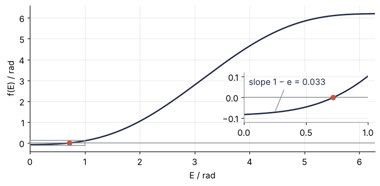
Kepler function f(E) in rad against E from 0 to 2π for M = 0.083 rad. It rises everywhere and crosses zero once, at E = 0.724 rad, where a dot marks the bracket. An inset zooms on E from 0 to 1 rad, where the curve starts almost flat below zero, with slope 0.033, and crosses at the root.

One sign change, a bracket 0.016 rad wide, drawn as the dot on the zero line. This scan is the general way to get a bracket for any continuous function: pick the range from the physics, evaluate on a grid, and it finds every root that crosses zero, as long as no two roots share a grid cell. A sign change can also be a pole, where \(f\) jumps from plus to minus infinity, and the square-well Variation shows how to tell the two apart.

The curve says two more things, both particular to Kepler. It rises everywhere, because \(f' = 1 - e\cos E \ge 1 - e > 0\), so there is exactly one root, and \([0, 2\pi]\) brackets it for any \(M\) in \([0, 2\pi)\). Near \(E = 0\) it is almost flat, with slope 0.033, and that is where Newton's method will get into trouble.

Step 2: Call brentq and turn E into a position

brentq takes the function, the two ends of the bracket, and the extra parameters as a tuple in args, passed after the unknown. The bracket is a contract: a continuous function that changes sign between the ends has a root inside, and Brent's method keeps it inside. It takes a faster step, along a curve through the last two or three points, when that step lands well inside the bracket and is shorter than half the step before last, and otherwise halves the bracket like bisection. With full_output=True it also returns what it did:

E1, res = brentq(kepler, 0, 2 * np.pi, args=(M1,), full_output=True)
print(f"E = {E1:.10f} rad\n")
print(res)

E = 0.7238907162 rad

      converged: True
           flag: converged
 function_calls: 15
     iterations: 14
           root: 0.7238907161951696
         method: brentq

Fourteen iterations and 15 calls of kepler, starting from the whole circle. converged is the field to read; the others are the cost.

In \(E\) the position is simple. With the Sun at the origin and perihelion on the positive \(x\) axis, \(x = a(\cos E - e)\), \(y = b\sin E\), and the distance is \(r = a(1 - e\cos E)\). The true anomaly \(\nu\) is the angle of the point \((x, y)\), and the orbit equation you know, \(r = p/(1 + e\cos\nu)\) with \(p = a(1 - e^2)\), makes a check:

x, y = a * (np.cos(E1) - e), b * np.sin(E1)
r = a * (1 - e * np.cos(E1))
nu = np.arctan2(y, x)
p = a * (1 - e**2)
print(f"r = {r:.6f} AU   nu = {np.degrees(nu):.1f}°   p/(1 + e cos nu) = {p / (1 + e * np.cos(nu)):.6f} AU")

r = 4.912502 AU   nu = 142.2°   p/(1 + e cos nu) = 4.912502 AU

The two distances agree to all six decimals, so \(E\) and \(\nu\) name the same point. One year after perihelion the comet is 4.91 AU out and has swung through 142° of its orbit, while \(M\) has moved by under 5°.

Step 3: Use the derivative with newton

Newton's method needs no bracket. It needs a starting value and, in its classic form, the derivative. From the start it follows the tangent to where it crosses zero and starts again from there. Once close, the number of correct digits roughly doubles with every step. For Kepler's equation the natural start is \(E_0 = M\), exact for a circle. Compare it with brentq, and with newton called without the derivative, one year after perihelion and 37 years after, near aphelion:

for t in (1.0, 37.0):
    M = mean_anomaly(t)
    _, rn = newton(kepler, M, fprime=kepler_prime, args=(M,), full_output=True)
    _, rs = newton(kepler, M, args=(M,), full_output=True)         # no fprime: secant
    _, rb = brentq(kepler, 0, 2 * np.pi, args=(M,), full_output=True)
    print(f"t = {t:4.1f} yr   newton {rn.iterations:2d} steps {rn.function_calls:2d} calls"
          f"   secant {rs.iterations:2d} steps {rs.function_calls:2d} calls"
          f"   brentq {rb.function_calls:2d} calls   converged: {rn.converged and rs.converged}")

t =  1.0 yr   newton  8 steps 16 calls   secant 12 steps 13 calls   brentq 15 calls   converged: True
t = 37.0 yr   newton  3 steps  6 calls   secant  3 steps  4 calls   brentq  8 calls   converged: True

Near aphelion Newton is done in three steps. Near perihelion it needs eight, because its first step overshoots on the flat part of the curve. Each Newton step calls both \(f\) and \(f'\), so compare calls, not steps: 16 for Newton against 15 for brentq at one year, six against eight at 37 years. Without fprime, newton runs the secant method, which takes the slope from the last two iterates instead of a derivative, and here it is the cheapest of the three, at 13 and four calls. Whichever you run, read converged.

Step 4: Choose between a bracket and a start, then switch with root_scalar

The choice depends on what you have. Use a bracket and brentq when you can find a sign change, from the physics (a quantity that must be positive at one end of the range and negative at the other) or from the grid scan of Step 1. It cannot diverge, needs no derivative, and cost 8 to 15 calls in Step 3. Use a start and newton when you have a good guess and a cheap derivative, when one call must solve a whole array of equations (brentq takes one bracket at a time), or when the root touches zero without crossing it, so that there is no sign change to find. A start comes from a physical approximation (\(E \approx M\) here), from the previous solution when you sweep a parameter, or from a grid point next to a sign change.

root_scalar puts both behind one interface, and a script switches between them by changing keywords:

print(root_scalar(kepler, args=(M1,), bracket=[0, 2 * np.pi], method="brentq"), "\n")
print(root_scalar(kepler, args=(M1,), x0=M1, fprime=kepler_prime, method="newton"))

      converged: True
           flag: converged
 function_calls: 15
     iterations: 14
           root: 0.7238907161951696
         method: brentq 

      converged: True
           flag: converged
 function_calls: 16
     iterations: 8
           root: 0.7238907161951694
         method: newton

The same root to 15 digits, and the same fields for every method: root, converged, flag, iterations, function_calls. Leave out method and root_scalar chooses; its documentation promises only that a bracket may lead to a bracketing method and a derivative with a start to a derivative-based one. Name the method, and you know what ran. If you have used minimize, converged plays the role of its success.

Step 5: Solve for a whole orbit at once and draw it

Give newton an array of starting values and an array of \(M\) in args, and it iterates on every element at once, because kepler is written in NumPy. The start changes for this. \(E_0 = M\) served one date at a time, but an array call does not stop when one element fails (Pitfalls), so it gets \(E_0 = \pi\), which converges for every \(M\) at any \(e < 1\), as the Pitfalls report. With full_output=True an array call returns three arrays: the roots, converged, and zero_der, which is True where the derivative hit zero and Newton could not take a step.

def solve_kepler(t_years):
    M = mean_anomaly(t_years)
    E, converged, zero_der = newton(kepler, np.full_like(M, np.pi), fprime=kepler_prime,
                                    args=(M,), full_output=True)
    assert converged.all() and not zero_der.any()
    return E

t_dots = np.arange(76.0)                          # years after perihelion
E_dots = solve_kepler(t_dots)
r_dots = a * (1 - e * np.cos(E_dots))
for t in (0, 1, 37, 38):
    print(f"t = {t:2d} yr   r = {r_dots[t]:5.2f} AU")
print(f"{np.sum(r_dots > 30)} of {t_dots.size} dots beyond 30 AU, {np.sum(r_dots < 5.2)} inside Jupiter's orbit")

t =  0 yr   r =  0.59 AU
t =  1 yr   r =  4.91 AU
t = 37 yr   r = 35.07 AU
t = 38 yr   r = 35.07 AU
35 of 76 dots beyond 30 AU, 3 inside Jupiter's orbit

All 76 converged. For the date, count back from the 2061 perihelion: 1 January is \(t = -208/365.25\) yr, and mean_anomaly wraps the negative angle to just below \(2\pi\). One date is a scalar call, with the same start.

t_2061 = -208 / 365.25
M_2061 = mean_anomaly(t_2061)
E_2061 = newton(kepler, np.pi, fprime=kepler_prime, args=(M_2061,))   # scalar call: raises if it fails
x_2061, y_2061 = a * (np.cos(E_2061) - e), b * np.sin(E_2061)
r_2061 = a * (1 - e * np.cos(E_2061))
print(f"M = {M_2061:.4f} rad   r on 1 January 2061 = {r_2061:.2f} AU")

M = 6.2357 rad   r on 1 January 2061 = 3.28 AU

Now the figure. The orbit line comes straight from a grid in \(E\), because the shape needs no dates; the dashed circles are the orbits of Earth and Jupiter, and an inset zooms on the inner solar system:

E_line = np.linspace(0, 2 * np.pi, 500)           # the shape alone needs no root
x_line, y_line = a * (np.cos(E_line) - e), b * np.sin(E_line)
x_dots, y_dots = a * (np.cos(E_dots) - e), b * np.sin(E_dots)
phi = np.linspace(0, 2 * np.pi, 200)

def draw(ax, ms):
    ax.plot(x_line, y_line, color=INK, lw=1)
    ax.plot(x_dots, y_dots, "o", color=ACCENT, ms=ms)
    for R in (1.0, 5.2):                          # Earth and Jupiter, for scale
        ax.plot(R * np.cos(phi), R * np.sin(phi), color=MUTED, lw=1, ls="--")
    ax.plot(0, 0, "*", color=INK, ms=10)
    ax.plot(x_2061, y_2061, "o", color=ACCENT, ms=9, mfc="white", mew=2)
    ax.set_aspect("equal")

fig, ax = plt.subplots(figsize=(8, 4.4))
draw(ax, ms=4)
ax.set(xlabel="x / AU", ylabel="y / AU", xlim=(-37, 6), ylim=(-6, 19))
ax.text(-35, 6, "aphelion: the dots crowd", color=INK)

axin = ax.inset_axes([-13, 8, 15, 11], transform=ax.transData)
draw(axin, ms=6)
axin.set(xlim=(-6.5, 6.5), ylim=(-6, 6))
axin.locator_params(nbins=3)                      # fewer ticks, not smaller labels
axin.spines[:].set_color(MUTED)
ax.indicate_inset_zoom(axin, edgecolor=MUTED, alpha=1)
axin.text(-6.3, 4.9, "Jupiter", color=MUTED)
axin.text(1.2, -1.9, "Earth", color=MUTED)
axin.text(1.3, 0.3, "Sun", color=INK)
ax.annotate(f"1 Jan 2061: r = {r_2061:.2f} AU", xy=(x_2061, y_2061), xytext=(-22, -1.6),
            color=ACCENT, arrowprops=dict(arrowstyle="-", color=ACCENT, lw=1))
plt.show()

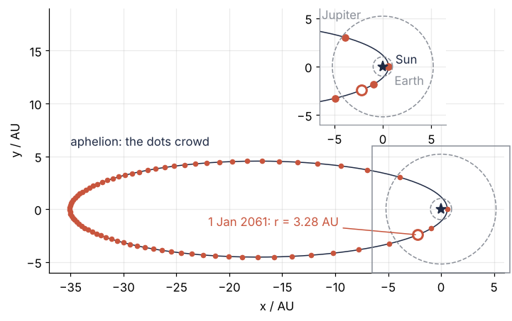
Orbit of Halley's comet in its plane, x and y in AU, Sun at the origin, with one dot per year after perihelion. The dots crowd at aphelion near x = -35 AU. A marker shows the comet 3.28 AU from the Sun on 1 January 2061, and an inset zooms on the inner 6 AU with the orbits of Earth and Jupiter.

In the model the comet is 3.28 AU from the Sun on 1 January 2061, inside Jupiter's orbit and coming in. Of the 76 yearly dots, 35 lie beyond 30 AU and only three inside Jupiter's orbit. That is the second law of the motivation made visible: near the Sun the line to the comet is short, so it must sweep a wide angle to cover the area it covers in a year at aphelion. The comet spends almost half its life farther out than Neptune.

Pitfalls

A bracket whose ends do not change sign. Give the 2061 date to brentq with an \(M\) that was never wrapped:

M_raw = 2 * np.pi * t_2061 / P
try:
    brentq(kepler, 0, 2 * np.pi, args=(M_raw,))
except ValueError as err:
    print(f"M = {M_raw:.4f} rad: ValueError: {err}")

M = -0.0475 rad: ValueError: f(a) and f(b) must have different signs

A negative time gives a negative \(M\), a time more than one period after perihelion gives one above \(2\pi\), and either way \(f\) has the same sign at both ends of \([0, 2\pi]\). Wrap with np.mod, as mean_anomaly does, or take the bracket \([M - e, M + e]\), which holds the root for any \(M\), because \(|E - M| = e|\sin E| \le e\).

A starting value where the slope is almost zero. Start Newton at perihelion, \(E_0 = 0\), where \(f' = 1 - e = 0.033\), for \(M = 1\) rad:

_, res0 = newton(kepler, 0.0, fprime=kepler_prime, args=(1.0,), full_output=True)
print(f"M = 1: first step to {0 - kepler(0.0, 1.0) / kepler_prime(0.0, 1.0):.1f} rad, "
      f"root {res0.root:.4f} rad after {res0.iterations} steps")

M = 1: first step to 30.3 rad, root 1.9114 rad after 13 steps

The first tangent shoots 30.3 rad out, almost five turns, and the call needs 13 steps to come back. That one recovered. Now start every \(M\) of a fine grid at zero in one array call, and catch the warning it issues:

M_grid = np.linspace(0, 2 * np.pi, 1001)[1:-1]
with warnings.catch_warnings(record=True) as caught:
    warnings.simplefilter("always")
    E_zero, ok_zero, _ = newton(kepler, np.zeros_like(M_grid), fprime=kepler_prime,
                                args=(M_grid,), maxiter=50, full_output=True)
print(f"warning: {caught[0].message}")
print(f"start E0 = 0: {np.sum(~ok_zero)} of {M_grid.size} failed")

warning: some failed to converge after 50 iterations
start E0 = 0: 163 of 999 failed

Of 999 values of \(M\), 163 do not converge within 50 iterations. Two other starts are at hand, the natural \(E_0 = M\) and \(E_0 = \pi\). To compare them as the orbit gets more eccentric, the eccentricity becomes a third argument of the function:

def kepler_e(E, M, ecc):
    return E - ecc * np.sin(E) - M

def kepler_e_prime(E, M, ecc):
    return 1 - ecc * np.cos(E)

for ecc in (0.967, 0.99):
    for name, E0 in (("M", M_grid), ("π", np.full_like(M_grid, np.pi))):
        with warnings.catch_warnings():
            warnings.simplefilter("ignore")
            _, ok, _ = newton(kepler_e, E0, fprime=kepler_e_prime, args=(M_grid, ecc),
                              maxiter=50, full_output=True)
        print(f"e = {ecc}   start E0 = {name}: {np.sum(~ok):3d} of {M_grid.size} failed")

e = 0.967   start E0 = M:   0 of 999 failed
e = 0.967   start E0 = π:   0 of 999 failed
e = 0.99   start E0 = M:  13 of 999 failed
e = 0.99   start E0 = π:   0 of 999 failed

\(E_0 = M\) is safe for Halley, but at \(e = 0.99\) it fails for 13 values. \(E_0 = \pi\) fails for none at either eccentricity, and Charles and Tatum (1998) showed that Newton's method from \(\pi\) converges for every \(M\) and every \(e < 1\). Start at \(\pi\), or use brentq.

Trusting newton without reading its flag. A scalar call that runs out of maxiter raises a RuntimeError, so you notice. An array call raises only when every element fails; the one above only warned, returned its last iterates, and went on. Some of those lie hundreds of radians or more from any sensible angle and are easy to spot, but not all:

E_true = np.array([brentq(kepler, 0, 2 * np.pi, args=(M,)) for M in M_grid])
wrong = ~ok_zero & (np.abs(E_zero - E_true) > 1e-6)
plausible = wrong & (E_zero > 0) & (E_zero < 2 * np.pi)
print(f"{np.sum(~ok_zero)} flagged, {np.sum(wrong)} wrong, {np.sum(plausible)} of them between 0 and 2π, for example")
for M, E, E_ok in zip(M_grid[plausible][:3], E_zero[plausible][:3], E_true[plausible][:3]):
    print(f"M = {M:.3f} rad   newton {E:.3f} rad   brentq {E_ok:.3f} rad")

163 flagged, 157 wrong, 26 of them between 0 and 2π, for example
M = 0.848 rad   newton 4.683 rad   brentq 1.792 rad
M = 1.319 rad   newton 2.434 rad   brentq 2.136 rad
M = 1.596 rad   newton 2.239 rad   brentq 2.310 rad

Of the 163 flagged elements 157 are wrong, and 26 of those lie between 0 and \(2\pi\), where they look like any other eccentric anomaly. A warning scrolls past in a long run, and a notebook may filter it. The fix is the check of Step 5: full_output=True and converged.all(), or root_scalar and its converged.

Variations

Several roots, as in the finite square well. The even bound states of a well of half-width \(w\) and depth \(V_0\) solve \(z\tan z = \sqrt{z_0^2 - z^2}\), where \(z\) is the wavenumber inside the well times \(w\) and \(z_0 = (w/\hbar)\sqrt{2mV_0}\) rolls depth and width into one number. Scan \((0, z_0)\) with the sign-change line of Step 1, call brentq on each bracket, and keep only the results where \(|f|\) is small. At \(z_0 = 8\) a 2,001-point grid finds six sign changes but three roots, 1.3955, 4.1648, and 6.8307. The other three are the poles of \(\tan z\) at \(\pi/2\), \(3\pi/2\), and \(5\pi/2\): brentq converges onto the jump, and \(|f|\) there is above \(10^{12}\) instead of below \(10^{-12}\).
Halley's method for Halley's comet. Add fprime2=lambda E, M: e * np.sin(E) to the newton call and it switches to Halley's method, which uses the second derivative too and, once close, roughly triples the number of correct digits with every step. Compare its steps with those of Step 3.
Hyperbolic orbits. For \(e > 1\) the equation becomes \(e\sinh H - H = M\) in the hyperbolic anomaly \(H\), with derivative \(e\cosh H - 1\), as for the interstellar object 'Oumuamua at \(e \approx 1.2\). \(M\) no longer wraps, so the bracket must grow with it.
Systems of equations. For several unknowns, such as the points where two coplanar orbits cross, scipy.optimize.root(fun, x0, jac=...) takes a vector function and its Jacobian, the matrix of partial derivatives.

Cheat sheet

i = np.nonzero(np.diff(np.sign(f(x_grid))))[0]          # brackets [x_grid[i], x_grid[i+1]]; check |f| at the result, poles flip sign too
x, r = brentq(f, lo, hi, args=(p,), full_output=True)    # needs a sign change; cannot diverge; r.converged
x = newton(f, x0, fprime=df, args=(p,))                  # start, derivative; f(x, p) and df(x, p) take the same args
x = newton(f, x0, args=(p,))                             # no fprime: secant;  fprime2=d2f: Halley
x, ok, zero_der = newton(f, x0_array, fprime=df, args=(p_array,), full_output=True)
assert ok.all()                                          # an array call warns when some fail, raises if all do
sol = root_scalar(f, args=(p,), bracket=[lo, hi], method="brentq")   # or x0=..., fprime=..., method="newton"
sol.root, sol.converged, sol.function_calls
M = np.mod(M, 2 * np.pi)                                 # Kepler: keep M in [0, 2π) for the bracket [0, 2π]