CT reconstruction with scikit-image: a head slice from its projections

The problem: what a CT scanner measures

A CT scanner never sees the slice it shows you. At each of a few hundred angles it sends rays through the head and measures the intensity \(I\) of every ray behind it against the intensity \(I_0\) without the head. CT reconstruction computes the slice from those numbers, and scikit-image has three functions to simulate and reconstruct it: radon, iradon, and iradon_sart. What links a measurement to the slice is the attenuation along the ray, Beer-Lambert's law:

with \(\mu\) the attenuation coefficient of the tissue and \(s\) the path along the ray. So \(-\ln(I/I_0)\) is the line integral of \(\mu\) along one ray. These logarithms, one per detector element and angle, are the sinogram: 72,000 numbers for a 400-element detector at 180 angles.

Whoever runs a scanner has to choose. How many angles, when each one costs dose and time? Which of the five filters that iradon offers? And when is an iterative method worth the extra run time?

The slice here is the Shepp-Logan head phantom that ships with scikit-image, ten ellipses of fixed attenuation on a 400 × 400 grid. Its sinogram is computed from those same pixels, so the data hold exactly what the reconstruction can represent: no detail finer than a pixel and no photon noise. Testing a method on data made by its own model is called the inverse crime, and every method looks better under it than on a scanner. From Step 4 on the data get noise. radon models parallel rays, as at a synchrotron beamline. Fan-beam data are rebinned to parallel rays first, and a laboratory micro-CT's cone beam needs a cone-beam code.

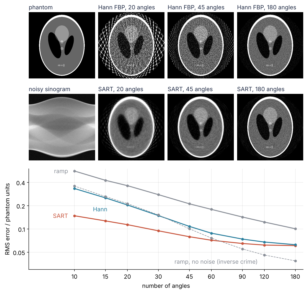
Step 6 draws it: noisy data reconstructed by the two methods the tutorial ends with, and their error against the number of angles.

Setup

To use your own slice, replace phantom. To use a measured sinogram, skip to Step 2 with the detector position on axis 0 and the angle on axis 1, converted from intensities first with -np.log(I / I0), where I0 is a flat-field scan without the object.

import warnings
import numpy as np
import matplotlib.pyplot as plt

warnings.filterwarnings("ignore", message="IProgress not found")   # skimage.data warns about a missing progress widget
from skimage.data import shepp_logan_phantom
from skimage.transform import radon, iradon, iradon_sart

plt.rcParams.update({
    "figure.figsize": (7, 3.6), "figure.dpi": 110,
    "axes.spines.top": False, "axes.spines.right": False,
    "axes.grid": True, "grid.alpha": 0.25,
    "font.size": 11, "lines.linewidth": 1.8,
})
INK, ACCENT, SECOND, MUTED = "#1f2a44", "#c8553d", "#2a7f9e", "#8a8f98"

phantom = shepp_logan_phantom()                   # skull 1.0, brain 0.2, inner ellipses 0 to 0.4
N = phantom.shape[0]
row, col = np.indices(phantom.shape)
inside = np.hypot(row - (N - 1) / 2, col - (N - 1) / 2) < N / 2   # radon's default circle=True sees only this disk

def rms_error(image):
    return np.sqrt(np.mean((image - phantom)[inside] ** 2))

SIGMA = 2.0                                       # noise per ray in sinogram units, 1.9 % of its largest value
rng = np.random.default_rng(1)

def add_noise(sino, sigma=SIGMA):
    return sino + sigma * rng.standard_normal(sino.shape)

def show(ax, image, label):
    """One gray scale for the phantom and every reconstruction: 0 to 0.5."""
    ax.imshow(image, cmap="gray", vmin=0, vmax=0.5)
    ax.text(0, 1.02, label, transform=ax.transAxes, va="bottom", color=INK)
    ax.set_axis_off()

print(phantom.shape, phantom.dtype, f"values {phantom.min():.1f} to {phantom.max():.1f}")

(400, 400) float64 values 0.0 to 1.0

Step 1: Simulate the sinogram with radon

radon takes an image and a list of angles in degrees and returns one projection per angle, the line integrals along all parallel rays at that angle. Take 180 angles spread evenly over half a turn. The other half would repeat them mirrored:

theta = np.linspace(0.0, 180.0, 180, endpoint=False)    # degrees
sinogram = radon(phantom, theta=theta)

column_sums = sinogram.sum(axis=0)
print("sinogram shape", sinogram.shape, "(detector position, angle)")
print(f"column sums {column_sums.min():.1f} to {column_sums.max():.1f}, phantom total {phantom.sum():.1f}")
print(f"largest line integral {sinogram.max():.1f}; SIGMA = {SIGMA} is {SIGMA / sinogram.max():.1%} of it")

sinogram shape (400, 180) (detector position, angle)
column sums 19703.2 to 19708.3, phantom total 19705.4
largest line integral 106.2; SIGMA = 2.0 is 1.9% of it

Each column sums to the phantom's total within 0.015 %: every projection carries the whole slice, seen from one side. The noise added from Step 4 on is 1.9 % of the largest line integral. For your scanner, scan one object twice: the standard deviation of the difference of the two sinograms, divided by \(\sqrt 2\), is the noise per ray, and divided by your largest line integral it is your counterpart of 1.9 %.

Copy

fig, (ax0, ax1) = plt.subplots(1, 2, figsize=(8, 3.6), width_ratios=[1, 1.4], layout="constrained")
show(ax0, phantom, "phantom")
ax1.imshow(sinogram, cmap="gray", aspect="auto", extent=[0, 180, N, 0])
ax1.set(xlabel="angle / degrees", ylabel="detector position / pixel", xticks=[0, 45, 90, 135, 180])
ax1.grid(False)
plt.show()

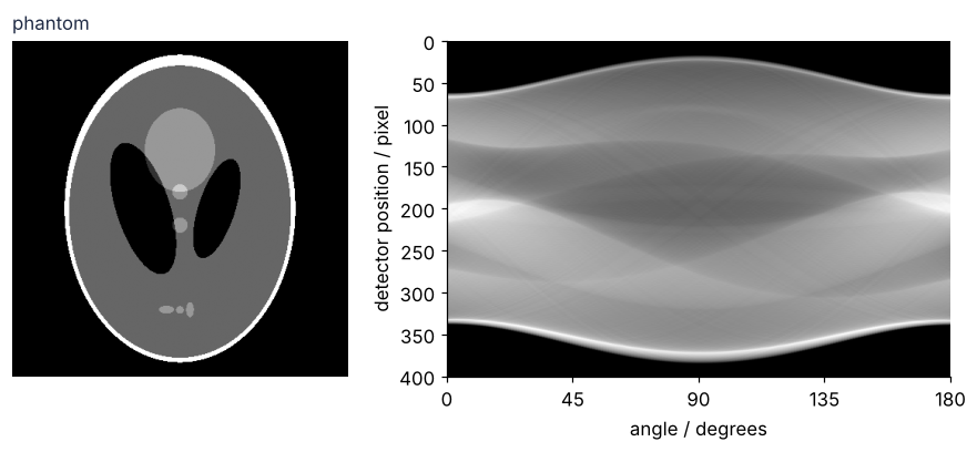
On the gray scale of 0 to 0.5 used for every image, the skull saturates and the brain's ellipses show. In the sinogram a single point of the slice lands on the detector at a position that swings like a sine as the angle turns, which gives the sinogram its name. The skull is the bright band, and the small ellipses are the faint sines inside it.

Step 2: Back-project, with and without the ramp filter

The obvious way back is to smear each projection across the image along the rays it was measured on and add up the smears from all angles. That is back projection. A single bright point comes back as a peak with a halo, because every smear passes through the point and the smears thin out with distance, as \(1/r\). A ramp filter removes the halo: before the smear it multiplies the Fourier transform of each projection by a weight proportional to the absolute frequency, which undoes the halo, because the \(1/r\) smear damps each spatial frequency \(f\) by \(1/|f|\) (the Fourier transform tutorial explains the transform). Back projection with this filter is filtered back projection, FBP, and clinical scanners have run variants of it for decades.

unfiltered = iradon(sinogram, theta=theta, filter_name=None)
fbp = iradon(sinogram, theta=theta)                       # filter_name="ramp" is the default
print(f"unfiltered   max {unfiltered.max():6.1f}")
print(f"ramp         max {fbp.max():6.2f}   RMS error {rms_error(fbp):.3f}")

unfiltered   max  116.5
ramp         max   1.08   RMS error 0.039

Copy

fig, (ax0, ax1) = plt.subplots(1, 2, figsize=(7, 3.4), layout="constrained")
im = ax0.imshow(unfiltered, cmap="gray")
ax0.text(0, 1.02, "no filter", transform=ax0.transAxes, va="bottom", color=INK)
ax0.set_axis_off()
fig.colorbar(im, ax=ax0, shrink=0.85, label="value / phantom units")
show(ax1, fbp, "ramp filter")
plt.show()

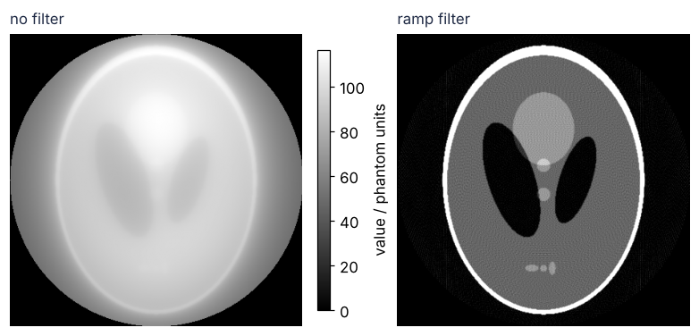
Unfiltered, the head is a blur with a maximum of 116.5 where the skull is 1.0. With the ramp it is sharp and back in phantom units, with an RMS error of 0.039, a fifth of the brain's value. That number is flattered by the inverse crime.

Step 3: Measure fewer angles, and the streaks they bring

Every angle is dose and time, so try fewer:

sparse = {}
for n in [20, 45, 90, 180, 360]:
    th = np.linspace(0.0, 180.0, n, endpoint=False)
    sparse[n] = iradon(radon(phantom, theta=th), theta=th)
    print(f"{n:4d} angles   RMS error {rms_error(sparse[n]):.3f}")

  20 angles   RMS error 0.213
  45 angles   RMS error 0.100
  90 angles   RMS error 0.055
 180 angles   RMS error 0.039
 360 angles   RMS error 0.035

Copy

fig, axes = plt.subplots(1, 2, figsize=(7, 3.4), layout="constrained")
for ax, n in zip(axes, [20, 45]):
    show(ax, sparse[n], f"{n} angles, RMS error {rms_error(sparse[n]):.3f}")
plt.show()

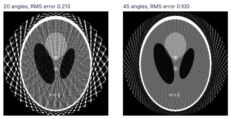
The error halves from 20 to 45 angles and barely moves above 180. With few angles the back-projected rays of the bright skull have no neighbors to cancel them, so straight streaks run off every edge. The usual rule for full sampling asks for about \(\pi/2 \times N\) angles for a detector of \(N\) elements, 628 here. It is written for the finest pattern the detector can hold. The phantom's ellipses are smooth, so above 180 angles only fine streaks near the edge are left, and the error moves by four thousandths.

Step 4: Add noise and choose the filter

The detector samples one value per pixel, so the finest pattern a projection can carry repeats every two pixels: 0.5 cycles per pixel, the Nyquist frequency, where the ramp is largest. Every other filter_name is the ramp multiplied by a window that is 1 at zero frequency and falls toward Nyquist. At Nyquist the Shepp-Logan window, a sinc, is down to 0.64, Hamming to 0.08, cosine and Hann to zero. scikit-image scales the ramp to reach 1 at Nyquist, which makes it \(2|f|\) with \(f\) in cycles per pixel, the same filter as in Step 2. Now add noise to the 180-angle sinogram and try all five:

noisy = add_noise(sinogram)
by_filter = {}
for name in ["ramp", "shepp-logan", "cosine", "hamming", "hann"]:
    by_filter[name] = iradon(noisy, theta=theta, filter_name=name)
    print(f"{name:12s} RMS error {rms_error(by_filter[name]):.3f}")

ramp         RMS error 0.100
shepp-logan  RMS error 0.085
cosine       RMS error 0.067
hamming      RMS error 0.063
hann         RMS error 0.063

Show code

Copy

f = np.linspace(0, 0.5, 200)                              # cycles per pixel
windows = {"shepp-logan": np.sinc(f), "cosine": np.cos(np.pi * f),
           "hamming": 0.54 + 0.46 * np.cos(2 * np.pi * f), "hann": 0.5 + 0.5 * np.cos(2 * np.pi * f)}

fig, axes = plt.subplots(1, 3, figsize=(8, 2.9), width_ratios=[1.3, 1, 1], layout="constrained")
ax = axes[0]
ax.plot(f, 2 * f, color=INK)
for name, w in windows.items():
    color = SECOND if name == "hann" else MUTED
    ax.plot(f, 2 * f * w, color=color, lw=1.8 if name == "hann" else 1.2)
label_at = {"ramp": (0.51, 1.0, "left", "center"), "shepp-logan": (0.51, 0.64, "left", "center"),
            "hamming": (0.51, 0.1, "left", "center"), "cosine": (0.28, 0.37, "center", "bottom"),
            "hann": (0.33, 0.03, "right", "bottom")}     # cosine and hann both end at 0: cosine at its top, hann below its arc
for name, (x, y, ha, va) in label_at.items():
    ax.text(x, y, name, color={"ramp": INK, "hann": SECOND}.get(name, MUTED), ha=ha, va=va)
ax.set(xlabel="frequency / cycles per pixel", ylabel="filter response", xlim=(0, 0.76), ylim=(0, 1.1),
       xticks=[0, 0.25, 0.5])
for ax, name in zip(axes[1:], ["ramp", "hann"]):
    show(ax, by_filter[name], f"{name}, RMS error {rms_error(by_filter[name]):.3f}")
plt.show()

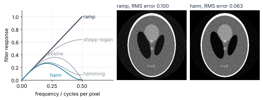
Noise drawn independently for every ray, as add_noise draws it, has the same strength at every frequency, which is what "white noise" means. The projections of a smooth head are strong at low frequencies and weak near Nyquist, so up there the ramp amplifies mostly noise. The windows that give away most of the upper half of the band win, and the ranking in the table follows the curves: Hann trades a slightly softer edge for an error of 0.063 instead of the ramp's 0.100. Use Hann, or Hamming, whenever the data are noisy, and the plain ramp only when the counts are high.

Step 5: Iterate with iradon_sart when the angles are few

SART, the simultaneous algebraic reconstruction technique, starts from a guess, projects it, and compares the projections with the measured sinogram. It spreads the difference back along the rays one angle at a time, damped by the default relaxation=0.15. One call of iradon_sart is one full pass over all angles, and that pass is what "an iteration" means here. iradon_sart writes each pass into the array passed as image and returns that same array, so the loop takes a .copy() of the second pass to keep it. Run six passes on noisy data at 20 and 45 angles, against Hann FBP on the same data:

results = {}
for n in [20, 45]:
    th = np.linspace(0.0, 180.0, n, endpoint=False)
    sino = add_noise(radon(phantom, theta=th))
    hann = iradon(sino, theta=th, filter_name="hann")
    recon, errors = None, []
    for k in range(6):
        recon = iradon_sart(sino, theta=th, image=recon)
        errors.append(rms_error(recon))
        if k == 1:
            two_passes = recon.copy()                     # recon is updated in place by the next pass
    results[n] = (hann, two_passes)
    print(f"{n} angles   Hann FBP {rms_error(hann):.3f}   SART passes 1 to 6:",
          " ".join(f"{e:.3f}" for e in errors))

20 angles   Hann FBP 0.204   SART passes 1 to 6: 0.137 0.114 0.105 0.101 0.100 0.099
45 angles   Hann FBP 0.108   SART passes 1 to 6: 0.100 0.079 0.074 0.074 0.075 0.077

Copy

fig, axes = plt.subplots(1, 2, figsize=(7, 3.4), layout="constrained")
hann, sart = results[20]
show(axes[0], hann, f"Hann FBP, RMS error {rms_error(hann):.3f}")
show(axes[1], sart, f"SART, 2 passes, RMS error {rms_error(sart):.3f}")
plt.show()

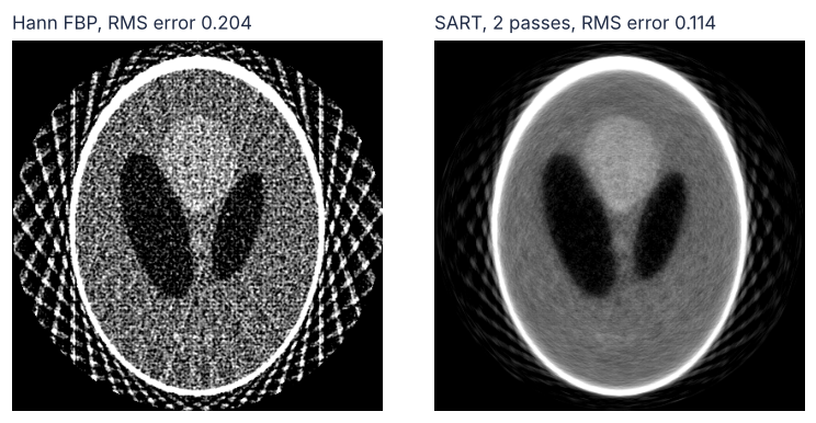
At 20 angles two passes cut the error of Hann FBP from 0.204 to 0.114, by 44 %, with weaker streaks and smoother noise. At 45 angles the error bottoms out after three or four passes and then rises, because SART starts fitting the noise; at 20 angles it only flattens. The second pass takes most of the gain, so two is the place to start, and the rest of this tutorial uses two. The price: one pass at 45 angles took about 0.5 s here, eight times as long as FBP.

Step 6: Sweep the number of angles, and where the methods cross

Repeat the comparison for angle counts from 10 to 180, with the noiseless ramp as the reference:

counts = [10, 15, 20, 30, 45, 60, 90, 120, 180]
curves = {"ramp, no noise": [], "ramp": [], "Hann": [], "SART": []}
images = {}
for n in counts:
    th = np.linspace(0.0, 180.0, n, endpoint=False)
    clean = radon(phantom, theta=th)
    sino = add_noise(clean)
    hann = iradon(sino, theta=th, filter_name="hann")
    sart = iradon_sart(sino, theta=th)
    sart = iradon_sart(sino, theta=th, image=sart)
    curves["ramp, no noise"].append(rms_error(iradon(clean, theta=th)))
    curves["ramp"].append(rms_error(iradon(sino, theta=th)))
    curves["Hann"].append(rms_error(hann))
    curves["SART"].append(rms_error(sart))
    images[n] = (sino, hann, sart)

print("angles " + "".join(f"{name:>16s}" for name in curves))
for n in [20, 45, 90, 180]:
    i = counts.index(n)
    print(f"{n:6d} " + "".join(f"{curves[name][i]:16.3f}" for name in curves))

angles   ramp, no noise            ramp            Hann            SART
    20            0.213           0.363           0.204           0.114
    45            0.100           0.212           0.108           0.079
    90            0.055           0.143           0.074           0.065
   180            0.039           0.101           0.063           0.061

SART leads at every count in the table, by 27 % at 45 angles, and Hann FBP closes in to 0.063 against 0.061 at 180: the curves meet near 180 angles. Whether that crossing belongs to the methods or to the noise shows when you run Hann and SART again at four times the noise, about 8 % of the largest line integral, and keep the error after one pass as well as after two:

print("4 x noise   Hann FBP   SART 1 pass   SART 2 passes")
for n in [45, 90, 180]:
    th = np.linspace(0.0, 180.0, n, endpoint=False)
    sino = add_noise(radon(phantom, theta=th), sigma=4 * SIGMA)
    hann = iradon(sino, theta=th, filter_name="hann")
    sart = iradon_sart(sino, theta=th)
    one_pass = rms_error(sart)                            # before the second pass overwrites sart
    sart = iradon_sart(sino, theta=th, image=sart)
    print(f"{n:4d} angles {rms_error(hann):9.3f} {one_pass:13.3f} {rms_error(sart):15.3f}")

4 x noise   Hann FBP   SART 1 pass   SART 2 passes
  45 angles     0.292         0.116           0.128
  90 angles     0.202         0.108           0.146
 180 angles     0.149         0.118           0.176

Copy

fig = plt.figure(figsize=(8, 7.6), layout="constrained")
grid = fig.add_gridspec(3, 4, height_ratios=[1, 1, 1.35])
show(fig.add_subplot(grid[0, 0]), phantom, "phantom")
ax = fig.add_subplot(grid[1, 0])
ax.imshow(images[180][0], cmap="gray", aspect="auto")
ax.set_box_aspect(1)                                      # as tall as the reconstructions beside it
ax.text(0, 1.02, "noisy sinogram", transform=ax.transAxes, va="bottom", color=INK)
ax.set_axis_off()
for j, n in enumerate([20, 45, 180], start=1):
    _, hann, sart = images[n]
    show(fig.add_subplot(grid[0, j]), hann, f"Hann FBP, {n} angles")
    show(fig.add_subplot(grid[1, j]), sart, f"SART, {n} angles")

ax = fig.add_subplot(grid[2, :])
styles = {"SART": dict(color=ACCENT), "Hann": dict(color=SECOND),
          "ramp": dict(color=MUTED), "ramp, no noise": dict(color=MUTED, ls="--", lw=1.0)}
for name, style in styles.items():
    ax.plot(counts, curves[name], marker="o", ms=4, **style)
ax.text(9.2, curves["ramp"][0], "ramp", color=MUTED, ha="right", va="center")
ax.text(9.2, curves["SART"][0], "SART", color=ACCENT, ha="right", va="center")
ax.text(14, 0.2, "Hann", color=SECOND, ha="center", va="top")
ax.text(110, 0.042, "ramp, no noise (inverse crime)", color=MUTED, ha="right", va="top")
ax.set(xscale="log", yscale="log", xlim=(5.5, 200), ylim=(0.03, 0.6),
       xlabel="number of angles", ylabel="RMS error / phantom units")
ax.set_xticks(counts, [str(n) for n in counts])
ax.set_yticks([0.05, 0.1, 0.2, 0.4], ["0.05", "0.1", "0.2", "0.4"])
ax.minorticks_off()
plt.show()

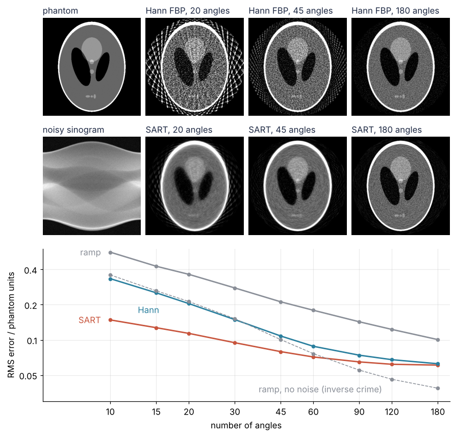
Where they meet, Hann is more than ten times faster: two SART passes at 180 angles took about 4 s here, FBP a quarter of a second. The dashed curve is what the inverse crime would have promised.

At 8 % noise the two-pass curves cross between 90 and 180 angles, and SART gets worse with more angles. Every pass makes one update per angle, so two passes at 180 angles are 360 updates against 90 at 45, and the extra updates fit noise, as the late passes of Step 5 did. One pass stays ahead of Hann at all three angle counts. With few angles, iterate, and stop earlier the noisier the data. Near the crossing, take Hann for its speed.

The crossing moves with the noise and with the detector size. To find yours, simulate a phantom on your detector's \(N\), set SIGMA in Setup to your fraction from Step 1 times the largest line integral Step 1 prints, rerun this sweep, and read off where the two curves meet.

Pitfalls

Angles in radians. The image comes out as parallel stripes with no head in them and an RMS error of 1.26 against 0.039. The cause is theta = np.linspace(0, np.pi, 180): radon and iradon read degrees, so all 180 projections fall within 3.14°. Write degrees and check that theta[-1] is close to 180 before you reconstruct anything.

Center of rotation off by a pixel or two. Edges turn ragged, the skull grows a faint second edge, and the error goes from 0.039 to 0.100 with the sinogram shifted by one pixel (np.roll(sinogram, 1, axis=0)) and to 0.151 with two. On a real scanner the rotation axis rarely falls on detector element N // 2, where iradon puts it. The projection at 180° is the one at 0° mirrored about the true axis. Record both, p0 and p180, with one extra projection if your angles stop short of 180°. Mirror p180 about element N // 2, which for even N is np.roll(p180[::-1], 1). Roll that copy by s from -10 to 10 pixels and keep the s with the smallest sum of squared differences from p0. The axis sits s / 2 pixels from N // 2, so shift the sinogram by -s / 2 along axis 0. An odd s means half a pixel, which np.roll cannot do, so use scipy.ndimage.shift(sinogram, (-s / 2, 0), order=1), which interpolates. Here one and two pixels off give s = 2 and 4, and the shift brings the error back to 0.039.

An object outside the circle. With the default circle=True, radon assumes the image is zero outside the inscribed circle and only issues a UserWarning when it is not, and the corners are lost from the sinogram. For an object that reaches the corners pass circle=False to both radon and iradon, which lengthens the detector to 566 elements for a 400 × 400 image, or pad the image with zeros.

Variations

• Limited angle. Take theta over 0° to 120° only, as in tomosynthesis or electron tomography. The missing wedge of angles blurs edges along one direction, and SART helps more there than any filter.
• Photon counts instead of Gaussian noise. Simulate counts = rng.poisson(I0 * np.exp(-mu * sinogram)), with mu the attenuation per pixel that a phantom value of 1 stands for, and take -np.log(counts / I0) / mu. The noise then gathers in the rays that graze the skull, where the fewest photons arrive.
• A 3D volume. Parallel-beam data reconstruct slice by slice, one iradon per detector row.
• Total variation after the reconstruction. skimage.restoration.denoise_tv_chambolle on a sparse-angle FBP or SART image removes streaks and noise while keeping edges, as in Denoise a low-light micrograph with scikit-image.

Cheat sheet

theta = np.linspace(0.0, 180.0, n, endpoint=False)         # degrees, never radians
sino = radon(image, theta=theta)                             # shape (detector, angle); circle=True by default
sino = -np.log(I / I0)                                       # measured intensities to line integrals first
img = iradon(sino, theta=theta, filter_name="hann")          # "ramp" default; "hamming", None
img = iradon(sino, theta=theta, circle=False, output_size=N) # object to the corners; size of the grid
x = None
for _ in range(2):                                           # SART: two passes to start, fewer if noisy
    x = iradon_sart(sino, theta=theta, image=x, relaxation=0.15)   # x is updated in place
sino = scipy.ndimage.shift(sino, (-s / 2, 0), order=1)       # s from the 0°/180° mirror test

Further reading

• The scikit-image API page of skimage.transform, for radon, iradon, and iradon_sart, and the gallery example Radon transform.
• Kak and Slaney, Principles of Computerized Tomographic Imaging (SIAM Classics, 2001), chapter 3 for filtered back projection and chapter 5 for the sampling rule; Buzug, Computed Tomography (Springer, 2008), for the scanner side.
• Shepp and Logan, "The Fourier reconstruction of a head section", IEEE Transactions on Nuclear Science 21 (1974), for the phantom; Andersen and Kak, "Simultaneous algebraic reconstruction technique (SART): a superior implementation of the ART algorithm", Ultrasonic Imaging 6 (1984), 81-94.
• Related tutorials on this site: MRI k-space reconstruction with numpy.fft: shifts, fold-over, ringing, the same kind of head from another measurement; Denoise a low-light micrograph with scikit-image: what each filter keeps, for total variation; The Fourier transform: asking a signal how much of each frequency it contains, for the filter. Planned: why the ramp filter is needed.
• Download the notebook. It was executed with the library versions in the header.