Derive a Jacobian with SymPy and pass it to solve_ivp with lambdify

The problem

You have the rate equations of a stiff system and want the implicit solver to get the exact Jacobian, not an estimate. Without jac, Radau in solve_ivp estimates it by finite differences, extra calls of the right-hand side that nfev does not count. SymPy derives the Jacobian without the sign errors of hand work, and lambdify makes it a NumPy function. The cell solves twice, with the estimate and with the SymPy Jacobian, and counts the calls of the right-hand side with a small wrapper.

The example is the Robertson reaction from \(y = (1, 0, 0)\) over 40 s, with \(k_1 = 0.04\) s⁻¹, and \(k_2 = 3 \times 10^7\) and \(k_3 = 10^4\) per unit of scaled concentration per second:

Swap in your own species, constants, rate equations, and plot scales; nothing else changes.

The code

Copy

import numpy as np
import sympy as sp
import matplotlib.pyplot as plt
from scipy.integrate import solve_ivp

# ---- your system: replace the species, the constants, the rate equations, and the plot scales
t = sp.Symbol("t")
y = A, B, C = sp.symbols("A B C")
k1, k2, k3 = sp.symbols("k1 k2 k3", positive=True)
rates = {k1: 0.04, k2: 3e7, k3: 1e4}       # 1/s; k2 and k3 per unit of scaled concentration per second
rhs = sp.Matrix([-k1 * A + k3 * B * C,
                 k1 * A - k3 * B * C - k2 * B**2,
                 k2 * B**2])
y0, t_span = [1.0, 0.0, 0.0], (0.0, 40.0)
plot_scale = {B: (1e4, "B × 10⁴")}          # species too small to see at scale 1; {} if none

# ---- the Jacobian
J = sp.simplify(rhs.jacobian(y))
print(J)

# ---- to NumPy
f = sp.lambdify((t, y), list(rhs.subs(rates)), "numpy")   # list: a flat vector, as solve_ivp wants
jac = sp.lambdify((t, y), J.subs(rates), "numpy")         # (t, y) even though t does not appear

# ---- solve twice, counting every call of f
def counted(fun):
    calls = [0]                               # a list, so that wrapper can add to it
    def wrapper(t_, y_):
        calls[0] += 1
        return fun(t_, y_)
    return wrapper, calls

runs = {}
for name, extra in [("finite differences", {}), ("SymPy Jacobian", {"jac": jac})]:
    f_counted, calls = counted(f)
    sol = runs[name] = solve_ivp(f_counted, t_span, y0, method="Radau", rtol=1e-6, atol=1e-10, **extra)
    print(f"{name:18s}  calls of f {calls[0]:4d}  nfev {sol.nfev:4d}  "
          f"Jacobians {sol.njev:2d}  steps {len(sol.t) - 1:2d}")
fd, sj = runs["finite differences"], runs["SymPy Jacobian"]
print(f"largest difference at {t_span[1]:g} s: {np.abs(fd.y[:, -1] - sj.y[:, -1]).max():.1e}")

# ---- plot: t = 0 is left out for the log axis
fig, ax = plt.subplots(figsize=(7, 3.6), dpi=110)
for i, s in enumerate(y):
    scale, label = plot_scale.get(s, (1, str(s)))
    ax.plot(sj.t[1:], scale * sj.y[i, 1:], "o-", color="#c8553d", ms=3, lw=1.6)
    ax.plot(fd.t[1:], scale * fd.y[i, 1:], "o", mfc="none", mec="#2a7f9e", ms=7, mew=1.1)
    ax.text(0.99, scale * sj.y[i, -1], label, color="#1f2a44", va="center",
            transform=ax.get_yaxis_transform())    # x in axes units, y in data units
ax.text(0.08, 0.66, "line and dots: SymPy Jacobian", color="#c8553d", transform=ax.transAxes)
ax.text(0.08, 0.57, "rings: finite differences", color="#2a7f9e", transform=ax.transAxes)
ax.set(xscale="log", xlabel="t / s", ylabel="concentration / initial A")
ax.spines[["top", "right"]].set_visible(False)
ax.grid(alpha=0.25)
plt.show()

Matrix([[-k1, C*k3, B*k3], [k1, -2*B*k2 - C*k3, -B*k3], [0, 2*B*k2, 0]])
finite differences  calls of f  703  nfev  647  Jacobians 18  steps 78
SymPy Jacobian      calls of f  647  nfev  647  Jacobians 18  steps 78
largest difference at 40 s: 1.2e-14

The knobs

lambdify writes the expression out as the source code of a Python function, with every SymPy function spelled as a function of some module, and then runs that source; inspect.getsource(jac), from the standard library, prints it. The modules argument picks that module. I give "numpy" explicitly, because without it lambdify takes SciPy first and NumPy second, so that a Bessel function lands in scipy.special. With cse=True, lambdify computes each common subexpression once, here the three products C*k3, B*k3, and 2*B*k2, which pays off when rate laws share denominators or the species run into the hundreds. simplify returns this Jacobian unchanged, because mass-action rate laws are polynomials, and earns its place on rational ones: the Michaelis-Menten rate \(V_\text{max} S / (K_m + S)\) differentiates to -S*V_max/(K_m + S)**2 + V_max/(K_m + S), which simplify turns into K_m*V_max/(K_m + S)**2. subs before lambdify fixes the constants. To vary them, in a fit or a temperature series, leave out subs, lambdify both rhs and J over (t, y, k) with k = (k1, k2, k3), and pass args=(k_values,) to solve_ivp, which hands that tuple to fun and jac alike.

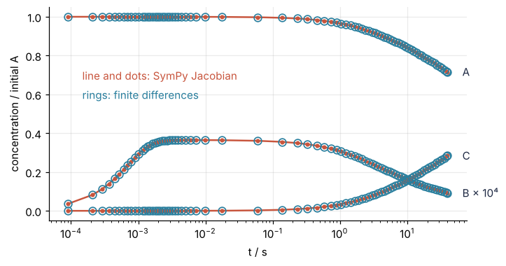
nfev reads 647 in both runs, while the wrapper counted 703 calls of f with finite differences and 647 with the SymPy Jacobian. The 56 calls in between, about 8 %, are the estimates, roughly one call per species for each of the 18 Jacobians. Nothing else moved: 78 steps and 18 Jacobians in both runs, and answers at 40 s that differ by 1.2 × 10⁻¹⁴, which the figure shows as a ring on every dot. The Jacobian feeds Radau's Newton iteration and the tolerances set the accuracy, so an exact Jacobian buys calls, not digits. The saving grows with the number of species times the number of Jacobian updates, and a mechanism with 300 species pays about 300 calls for every Jacobian. The printed matrix is the one the stiffness tutorial wrote by hand, entry for entry.

Pitfalls

A Matrix where solve_ivp wants a flat list. Lambdify the Matrix rhs itself and the right-hand side returns a (3, 1) column, which solve_ivp cannot store:

f_column = sp.lambdify((t, y), rhs.subs(rates), "numpy")
try:
    solve_ivp(f_column, t_span, y0, method="Radau")
except ValueError as err:
    print("ValueError:", err)

ValueError: could not broadcast input array from shape (3,1) into shape (3,)

The fix is list(rhs), as in the code. The Jacobian may stay a Matrix: it becomes the (3, 3) array that jac should return.

A symbol named like something in the generated code. Chemistry has a species called e, the electron of plasma and electrochemical mechanisms, and the generated source spells Euler's number e as well:

import inspect

e = sp.Symbol("e")
times_euler = sp.lambdify(e, e * sp.E, "numpy")
print(times_euler(2.0))
print(inspect.getsource(times_euler))
electron = sp.Symbol("electron")
print(sp.lambdify(electron, electron * sp.E, "numpy")(2.0))

4.0
def _lambdifygenerated(e):
    return e*e

5.43656365691809

The first result is 4.0 where 2e = 5.44 is right, and the source shows why: return e*e, the argument times itself, with no warning. A symbol named exp or sqrt at least fails loudly, with TypeError: 'float' object is not callable. Rename the symbol. The string counts, not the Python variable, and sp.Symbol("electron") gives 5.44.

A Jacobian that does not take (t, y). Lambdified over y alone, the Jacobian is a function of A, B, and C, and the reverse order (y, t) breaks the right-hand side instead:

jac_y = sp.lambdify(y, J.subs(rates), "numpy")
f_yt = sp.lambdify((y, t), list(rhs.subs(rates)), "numpy")
for fun, jac_try in [(f, jac_y), (f_yt, None)]:
    try:
        solve_ivp(fun, t_span, y0, method="Radau", jac=jac_try)
    except TypeError as err:
        print("TypeError:", err)

TypeError: _lambdifygenerated() missing 1 required positional argument: 'C'
TypeError: cannot unpack non-iterable float object

Always write (t, y), with y the tuple of symbols, even when t does not appear. That mirrors how solve_ivp calls both functions, a number t and then one array y, which the generated function unpacks into A, B, and C.