Tikhonov regularization: why undoing a blur amplifies the noise

The question

A spectrum has three peaks on 200 samples: one at sample 60, and a close pair at 110 and 124. The instrument blurs it with a Gaussian of standard deviation 3 samples and adds white noise of 0.001, a thousandth of the tallest peak. The blur is a matrix. Row i of A holds the Gaussian centered on sample i, normalized to sum 1, so \((Af)_i\) is a weighted average of the true spectrum f around sample i, and the measurement is b = Af plus the noise. A is invertible, so Ax = b has exactly one solution, and np.linalg.solve returns it:

Show code

Copy

import numpy as np
import matplotlib.pyplot as plt
from scipy.optimize import brentq

plt.rcParams.update({
    "figure.figsize": (7, 3.6), "figure.dpi": 110,
    "axes.spines.top": False, "axes.spines.right": False,
    "axes.grid": True, "grid.alpha": 0.25,
    "font.size": 11, "lines.linewidth": 1.8,
})
INK, ACCENT, SECOND, MUTED = "#1f2a44", "#c8553d", "#2a7f9e", "#8a8f98"
norm = np.linalg.norm

# The spectrum is synthetic, so that the answer can be checked at the end.
# Pretend you have not seen this cell.
N, sigma_blur, sigma_noise = 200, 3.0, 1e-3
idx = np.arange(N)
peaks = [60, 110, 124]


def peak(center, width, height):
    return height * np.exp(-0.5 * ((idx - center) / width) ** 2)


f_true = peak(60, 4, 1.0) + peak(110, 3, 0.6) + peak(124, 3, 0.8)
A = np.exp(-0.5 * ((idx[:, None] - idx[None, :]) / sigma_blur) ** 2)
A /= A.sum(axis=1, keepdims=True)                 # each row a weighted average
rng = np.random.default_rng(115)
b_clean = A @ f_true
b = b_clean + sigma_noise * rng.standard_normal(N)

x_naive = np.linalg.solve(A, b)
kappa = np.linalg.cond(A)
print(f"κ(A) = {kappa:.2g},  max |x_naive| = {np.abs(x_naive).max():.2g}")
for p in peaks:
    print(f"peak at {p:3d}:  true {f_true[p]:.3f},  measured {b[p]:.3f}  ({100 * (b[p] / f_true[p] - 1):+.0f} %)")
print(f"dip between the pair: true {f_true[110:125].min():.2f},  measured {b_clean[110:125].min():.2f}")

fig, (ax1, ax2) = plt.subplots(2, 1, figsize=(7, 4.6), sharex=True)
ax1.plot(idx, f_true, color=INK, lw=1.4)
ax1.plot(idx, b, color=SECOND)
ax1.text(66, 0.95, "truth", color=INK, ha="left")
ax1.text(66, 0.6, "measured", color=SECOND, ha="left")
ax1.set(ylabel="intensity / a.u.", ylim=(-0.1, 1.15))
ax2.plot(idx, x_naive / 1e13, color=ACCENT, lw=0.8)
ax2.text(0.01, 0.96, "np.linalg.solve(A, b)", transform=ax2.transAxes, ha="left", va="top", color=ACCENT)
ax2.set(xlabel="sample", ylabel="x / 10¹³", xlim=(0, N - 1))
plt.show()

κ(A) = 3.6e+17,  max |x_naive| = 1.2e+13
peak at  60:  true 1.000,  measured 0.799  (-20 %)
peak at 110:  true 0.600,  measured 0.425  (-29 %)
peak at 124:  true 0.800,  measured 0.568  (-29 %)
dip between the pair: true 0.09,  measured 0.25

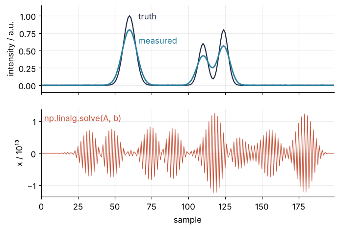
The measured peaks are 20 to 29 % lower than the true ones and wider, and the dip between the pair has filled from 0.09 to 0.25. The exact solution looks like nothing at all. It swings between plus and minus 1.2 × 10¹³ (around 10¹³; the last digits depend on the LAPACK build behind your NumPy), and the peaks are lost in it. The condition number of A is 3.6 × 10¹⁷, so the solve was expected to fail, but κ is one number for the whole matrix. Why does noise at a thousandth turn into 10¹³, and which part of the original spectrum can the data give back at all?

The idea: the blur damps fine detail, and the inverse undoes it on the noise too

The condition number pictured the singular values as the half-axes of the ellipse into which A turns the unit circle. The full statement is the singular value decomposition, \(A = U\Sigma V^\mathsf{T}\). The columns \(v_i\) of V are orthonormal patterns in the space of spectra, the columns \(u_i\) of U orthonormal patterns in the space of data, and \(A v_i = \sigma_i u_i\): A takes the pattern \(v_i\) to the pattern \(u_i\) and shrinks it by \(\sigma_i\). Any spectrum is a sum of the \(v_i\), so A acts on each of its components separately. The singular value decomposition treats all of this in full; here is what the patterns look like for the blur:

Show code

Copy

U, s, Vt = np.linalg.svd(A)
for i in [1, 10, 40, 100, 200]:
    print(f"σ_{i:<3d} = {s[i - 1]:.2g}")
print(f"σ_min / σ_max = {s[-1] / s[0]:.2g},  {np.sum(s < 1e-15 * s[0])} of {N} below 1e-15 σ_max")

def sub(i):
    return str(i).translate(str.maketrans("0123456789", "₀₁₂₃₄₅₆₇₈₉"))


def sci(v):
    """2.6e-05 as 2.6 × 10⁻⁵, for labels."""
    m, e = f"{v:.1e}".split("e")
    return f"{v:#.2g}" if v >= 0.01 else f"{m} × 10" + str(int(e)).translate(str.maketrans("-0123456789", "⁻⁰¹²³⁴⁵⁶⁷⁸⁹"))


fig, axes = plt.subplots(4, 1, figsize=(7, 6), sharex=True)
for ax, i in zip(axes, [1, 10, 40, 100]):
    ax.plot(idx, Vt[i - 1], color=INK, lw=1.2)
    ax.text(0.99, 0.97, f"v{sub(i)},  σ = {sci(s[i - 1])}", transform=ax.transAxes, ha="right", va="top")
    ax.set(ylim=(-0.17, 0.27), yticks=[-0.1, 0, 0.1])
axes[-1].set(xlabel="sample", xlim=(0, N - 1))
fig.supylabel("component", fontsize=11)
plt.show()

σ_1   = 1
σ_10  = 0.91
σ_40  = 0.19
σ_100 = 2.6e-05
σ_200 = 2.3e-17
σ_min / σ_max = 2.3e-17,  21 of 200 below 1e-15 σ_max

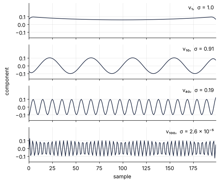
The pattern with the largest singular value, \(\sigma_1 = 1.0\), is a smooth hump that the blur passes almost untouched. At \(v_{10}\) the pattern has a few slow waves and \(\sigma_{10} = 0.91\). At \(v_{40}\) the waves are a dozen samples long and the blur keeps a fifth of their amplitude, \(\sigma_{40} = 0.19\). At \(v_{100}\) the pattern alternates every few samples, and a Gaussian average over 3 samples wipes it out down to \(\sigma_{100} = 2.6 \times 10^{-5}\). The smallest, \(\sigma_{200}\), is \(2.3 \times 10^{-17}\) of the largest, and 21 of the 200 are below \(10^{-15}\) of it.

So the blur multiplies each component of the spectrum by its \(\sigma_i\), and fine detail comes out of the instrument multiplied by almost nothing. Solving the system divides each component by \(\sigma_i\) again. That would restore the spectrum exactly if the data held only the blurred spectrum. They also hold the noise, and white noise has the same size, about \(10^{-3}\), in every direction, the fast patterns included. Divided by \(\sigma_{200}\), a \(10^{-3}\) becomes \(10^{13}\). The solve did what it was asked; the question was wrong.

The Picard plot: which details the data carry

Because the \(u_i\) are orthonormal, the coefficient \(u_i^\mathsf{T} b\) is how much of the data pattern \(u_i\) the measurement contains, and dividing it by \(\sigma_i\) gives the amount of \(v_i\) in the solution. Plot both \(\sigma_i\) and \(|u_i^\mathsf{T} b|\) against i on a logarithmic scale, and you see which components the data carry:

Show code

Copy

i_all = np.arange(1, N + 1)
beta = U.T @ b
beta_clean = U.T @ b_clean
i_cross = i_all[np.abs(beta_clean) < sigma_noise][0]
sigma_hat = np.sqrt(np.mean(beta[100:] ** 2))     # the flat tail, i = 101 to 200, chosen by eye
print(f"noise-free coefficients fall below the noise level at i = {i_cross}")
print(f"noise level from the floor: {sigma_hat:.2g}  (true {sigma_noise:.2g})")
print(f"largest |u_iᵀb| / σ_i: {np.max(np.abs(beta) / s):.1g}")


def picard(ax):
    ax.axvspan(101, 200, color=MUTED, alpha=0.12, lw=0)
    ax.axhline(sigma_noise, color=MUTED, lw=1, ls="--")
    ax.semilogy(i_all, s, color=INK)
    ax.semilogy(i_all, np.abs(beta_clean), color=SECOND, lw=1, alpha=0.35)
    ax.semilogy(i_all, np.abs(beta), "o", color=SECOND, ms=3)
    ax.text(155, 2e-6, "|uᵢᵀb|", color=SECOND, va="bottom")
    ax.text(62, 1e-11, "noise-free", color=SECOND, alpha=0.6)
    ax.text(165, 1e-11, "σᵢ", color=INK)
    ax.text(3, 6e-4, "noise level", color=MUTED, va="top")
    ax.set(xlabel="index i", ylabel="size", xlim=(0, 201), ylim=(1e-18, 10))


fig, ax = plt.subplots(figsize=(7, 3.6))
picard(ax)
ax.annotate(f"i = {i_cross}", (i_cross, sigma_noise), xytext=(25, 1e-8), color=SECOND,
            arrowprops=dict(arrowstyle="-", color=SECOND, lw=0.8))
plt.show()

noise-free coefficients fall below the noise level at i = 43
noise level from the floor: 0.00092  (true 0.001)
largest |u_iᵀb| / σ_i: 4e+13

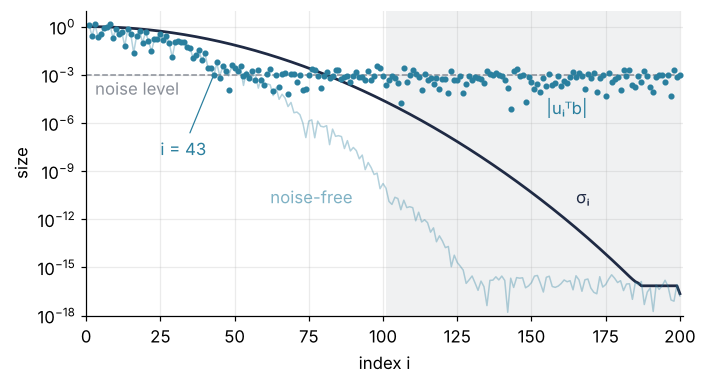
The coefficients fall with the singular values until they reach the noise level, \(10^{-3}\), at i = 43, and stay there while the singular values fall another sixteen decades. For about a dozen indices past it, signal and noise are of the same size; beyond those, the data carry noise and nothing else, and \(|u_i^\mathsf{T} b|/\sigma_i\) climbs to \(4 \times 10^{13}\). The faint curve is what noise-free data would show, still falling. A solution can be recovered only where the coefficients fall faster than the singular values; that requirement is the Picard condition.

The floor is useful on its own. Because U is orthogonal, white noise of standard deviation \(\sigma_\text{noise}\) puts the same typical size \(\sigma_\text{noise}\) into every coefficient, so the height of the floor is the noise level, readable off your own Picard plot with no truth at hand. The root mean square over the shaded tail, chosen well past the crossover, gives \(0.92 \times 10^{-3}\) against the true \(10^{-3}\). This holds for white noise only; when each measurement has its own standard deviation, divide its row of A and its entry of b by it first, and the noise becomes white with level 1.

A penalty on size

The naive solution fits the data to the last digit and is \(10^{13}\) large. Ask for something else: an x that fits the data well and is not too large. The weight of the second wish is a number λ, measured on the same scale as the singular values, and it damps the components with \(\sigma_i\) well below λ while keeping those well above. A λ of 0.038 means keeping what the components with \(\sigma_i\) above about 0.04 carry. Here are three settings:

Show code

Copy

def tikhonov(lam, beta=beta):
    """Regularized solution through the filter factors; beta = Uᵀb."""
    return Vt.T @ (s**2 / (s**2 + lam**2) * beta / s)


def rel_err(x):
    return norm(x - f_true) / norm(f_true)


def residual(lam):
    return norm(A @ tikhonov(lam) - b)


lam_dp = 10 ** brentq(lambda t: residual(10**t) - sigma_noise * np.sqrt(N), -6, 0)   # see Formalization
settings = [1e-4, lam_dp, 0.3]

fig, axes = plt.subplots(3, 1, figsize=(7, 6), sharex=True)
for ax, lam in zip(axes, settings):
    x = tikhonov(lam)
    print(f"λ = {lam:6.2g}:  relative error {100 * rel_err(x):6.1f} %,  "
          f"peaks {', '.join(f'{100 * (x[p] / f_true[p] - 1):+.0f} %' for p in peaks)}")
    ax.plot(idx, f_true, color=INK, lw=1.4)
    ax.plot(idx, np.clip(x, -0.45, 1.45), color=ACCENT, lw=1.4)
    clipped = ",  clipped" if np.abs(x).max() > 1.45 else ""
    ax.text(0.99, 0.97, f"λ = {lam:.2g},  error {100 * rel_err(x):.2g} %{clipped}" if rel_err(x) < 1 else
            f"λ = {lam:.2g},  error {100 * rel_err(x):.0f} %{clipped}", transform=ax.transAxes,
            ha="right", va="top")
    ax.set(ylim=(-0.5, 1.95), yticks=[0, 0.5, 1], ylabel="intensity / a.u.")
axes[-1].text(3, 1.0, "truth", color=INK)
axes[-1].text(3, 0.55, "Tikhonov", color=ACCENT)
axes[-1].set(xlabel="sample", xlim=(0, N - 1))
plt.show()

λ = 0.0001:  relative error  581.1 %,  peaks +33 %, -259 %, +113 %
λ =  0.038:  relative error    1.9 %,  peaks -1 %, -2 %, -1 %
λ =    0.3:  relative error   15.7 %,  peaks -16 %, -23 %, -23 %

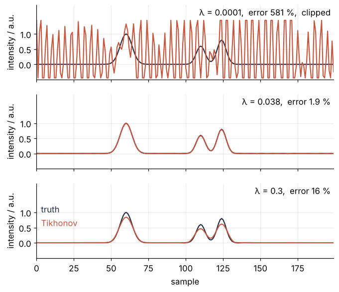
At λ = 10⁻⁴ the penalty keeps the 93 components with \(\sigma_i\) above \(10^{-4}\), fifty of them past the noise floor, and the solution is 581 % off. At λ = 0.038, a value whose origin is the next section's business, the solution lies on the truth within 1.9 %, and the pair is two peaks with a deep dip between them. At λ = 0.3 the penalty eats into components the data did carry, the peaks come out 16 to 23 % low, and the error is 16 %. Too little penalty and the noise wins; too much and the blur wins again.

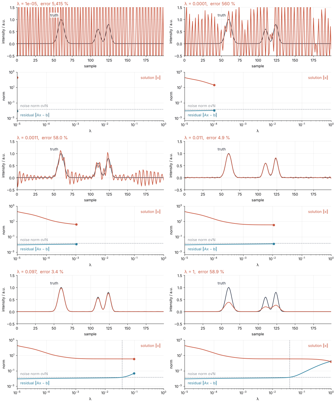
Now let λ run from \(10^{-5}\) to 1:

"""Lambda sweep: Tikhonov regularization of a blurred spectrum, from too little to too much.

Renders ../../assets/lambda-sweep.gif for the Tikhonov tutorial. The data are rebuilt with the
same lines and the same seed as the tutorial's setup cell. The penalty lambda sweeps from 1e-5
to 1 and pauses where the residual meets the noise norm. Top: the true spectrum and the
regularized one. Bottom: the norms of the residual and of the solution against lambda, with
the expected noise norm dashed. Run it from any directory:

    python scene.py
"""
from pathlib import Path

import numpy as np
import matplotlib.pyplot as plt
from matplotlib.animation import FuncAnimation, PillowWriter
from PIL import Image, ImageSequence
from scipy.optimize import brentq

OUT = Path(__file__).resolve().parents[2] / "assets" / "lambda-sweep.gif"
INK, ACCENT, SECOND, MUTED = "#1f2a44", "#c8553d", "#2a7f9e", "#8a8f98"
plt.rcParams.update({"axes.spines.top": False, "axes.spines.right": False,
                     "axes.grid": True, "grid.alpha": 0.25, "font.size": 11})

# ---- data: the same spectrum, blur, and noise as in the tutorial
N, sigma_blur, sigma_noise = 200, 3.0, 1e-3
idx = np.arange(N)


def peak(center, width, height):
    return height * np.exp(-0.5 * ((idx - center) / width) ** 2)


f_true = peak(60, 4, 1.0) + peak(110, 3, 0.6) + peak(124, 3, 0.8)
A = np.exp(-0.5 * ((idx[:, None] - idx[None, :]) / sigma_blur) ** 2)
A /= A.sum(axis=1, keepdims=True)
rng = np.random.default_rng(115)
b = A @ f_true + sigma_noise * rng.standard_normal(N)

U, s, Vt = np.linalg.svd(A)
beta = U.T @ b


def tikhonov(lam):
    """Regularized solution through the filter factors."""
    return Vt.T @ (s**2 / (s**2 + lam**2) * beta / s)


noise_norm = sigma_noise * np.sqrt(N)
lam_fine = np.logspace(-5, 0, 401)
res_fine = np.array([np.linalg.norm(A @ tikhonov(lam) - b) for lam in lam_fine])
sol_fine = np.array([np.linalg.norm(tikhonov(lam)) for lam in lam_fine])
log_dp = brentq(lambda t: np.linalg.norm(A @ tikhonov(10**t) - b) - noise_norm, -6, 0)

# 90 frames: the sweep, with ten extra frames held where the residual meets the noise
sweep = np.linspace(-5, 0, 80)
k = np.searchsorted(sweep, log_dp)
frames = 10 ** np.concatenate([sweep[:k], np.full(10, log_dp), sweep[k:]])

# ---- figure, drawn once
fig, (ax1, ax2) = plt.subplots(2, 1, figsize=(7, 5.6), dpi=80, layout="constrained")
ax1.plot(idx, f_true, color=INK, lw=1.4)
(x_line,) = ax1.plot([], [], color=ACCENT, lw=1.6)
ax1.text(56, 1.12, "truth", color=INK, ha="right", zorder=3,             # readable over a wild solution
         bbox=dict(facecolor="white", edgecolor="none", alpha=0.85, pad=1))
ax1.set(xlim=(0, N - 1), ylim=(-0.5, 1.5), xlabel="sample", ylabel="intensity / a.u.")
title = ax1.set_title("", loc="left", color=ACCENT)                   # names the red curve

ax2.axhline(noise_norm, color=MUTED, lw=1, ls="--")
dp_mark = ax2.axvline(10**log_dp, color=MUTED, lw=1, ls="--", visible=False)   # shown once reached
ax2.text(1.3e-5, noise_norm * 1.5, "noise norm σ√N", color=MUTED, va="bottom")
(res_trace,) = ax2.plot([], [], color=SECOND, lw=1.8)
(sol_trace,) = ax2.plot([], [], color=ACCENT, lw=1.8)
(res_dot,) = ax2.plot([], [], "o", color=SECOND, ms=6)
(sol_dot,) = ax2.plot([], [], "o", color=ACCENT, ms=6)
ax2.text(1.3e-5, 5e-3, "residual ‖Ax − b‖", color=SECOND, va="top")
ax2.text(0.98, 0.93, "solution ‖x‖", transform=ax2.transAxes, color=ACCENT, ha="right", va="top")
ax2.set(xscale="log", yscale="log", xlim=(1e-5, 1), ylim=(5e-4, 1e3), xlabel="λ", ylabel="norm")


# ---- one frame: a function of lambda alone
def update(lam):
    x = tikhonov(lam)
    x_line.set_data(idx, np.clip(x, -0.6, 1.6))       # clipped so a wild solution stays a band
    err = np.linalg.norm(x - f_true) / np.linalg.norm(f_true)
    title.set_text(f"λ = {lam:.2g},  error {100 * err:,.0f} %" if err > 1 else f"λ = {lam:.2g},  error {100 * err:.1f} %")
    shown = lam_fine <= lam
    res_trace.set_data(lam_fine[shown], res_fine[shown])
    sol_trace.set_data(lam_fine[shown], sol_fine[shown])
    res_dot.set_data([lam], [np.linalg.norm(A @ x - b)])
    sol_dot.set_data([lam], [np.linalg.norm(x)])
    dp_mark.set_visible(lam >= 10**log_dp)


# ---- render, and read back what was written
OUT.parent.mkdir(exist_ok=True)
FuncAnimation(fig, update, frames=frames).save(OUT, writer=PillowWriter(fps=12))
plt.close(fig)
with Image.open(OUT) as im:                          # Pillow merges the held frames into one
    seconds = sum(frame.info["duration"] for frame in ImageSequence.Iterator(im)) / 1000
    print(f"{OUT.name}: {im.width} x {im.height} px, {im.n_frames} frames, "
          f"{seconds:.1f} s, {OUT.stat().st_size / 1024:,.0f} kB")

The residual \(\|Ax - b\|\), how far the solution misses the data, creeps up with λ. Near λ = 0.038 it reaches the size of the noise itself, \(\sigma_\text{noise}\sqrt{N}\), the dashed line, and that is where the spectrum looks right: the solution misses the data by as much as the true spectrum does, no less and no more.