The singular value decomposition: how many species hide in a matrix of spectra
Afterwards you can explain what the singular value decomposition does, read a matrix's effective rank from its singular values, and denoise data by truncation.
- Topic
- Linear algebra
- Field
- Chemistry, Physics
- Prerequisites
- Eigenvalues with numpy.linalg: normal modes of coupled oscillators, PCA with scikit-learn: sixty absorption spectra in two dimensions
- Libraries
matplotlib 3.11.2numpy 2.4.3
py-svd.ipynb, executed with the versions above. The download needs a free account
Run it yourself. In a terminal, this installs exactly the versions above:
pip install numpy==2.4.3 matplotlib==3.11.2 jupyterlabThe question
A pump pulse excites a dye at time zero, and a white-light probe measures the change in absorbance, ΔA, at 300 wavelengths from 400 to 699 nm, after each of 200 delays from 0 to 597 ps. That is a transient absorption experiment, and its record is a matrix: 200 rows of delays, 300 columns of wavelengths, 60,000 numbers in mOD, thousandths of an absorbance unit. The singular value decomposition is the tool that reads off such a matrix how many species are in it.
Show code
import numpy as np
import matplotlib.pyplot as plt

plt.rcParams.update({
    "figure.figsize": (8, 3.4), "figure.dpi": 110,
    "axes.spines.top": False, "axes.spines.right": False,
    "axes.grid": True, "grid.alpha": 0.25,
    "font.size": 11, "lines.linewidth": 1.8,
})
INK, ACCENT, SECOND, MUTED = "#1f2a44", "#c8553d", "#2a7f9e", "#8a8f98"

# The record is synthetic, two species with sequential kinetics A -> B -> ground state
# plus white noise, so that the answer can be checked at the end. Pretend you have not seen this cell.
rng = np.random.default_rng(198)
t = np.arange(200) * 3.0                               # delay / ps
wl = np.arange(400, 700, 1.0)                          # wavelength / nm
k1, k2 = 1 / 40, 1 / 250                               # rate constants / ps^-1
c_A = np.exp(-k1 * t)
c_B = k1 / (k2 - k1) * (np.exp(-k1 * t) - np.exp(-k2 * t))
s_A = 5.0 * np.exp(-0.5 * ((wl - 470) / 30) ** 2)      # mOD
s_B = 3.0 * np.exp(-0.5 * ((wl - 540) / 40) ** 2)
D_true = np.outer(c_A, s_A) + np.outer(c_B, s_B)
D = D_true + 1.0 * rng.standard_normal(D_true.shape)
print(f"D: {D.shape[0]} delays x {D.shape[1]} wavelengths")

extent = [wl[0], wl[-1], t[0], t[-1]]
fig, (ax1, ax2) = plt.subplots(1, 2, layout="constrained", width_ratios=[1.15, 1])
fig.get_layout_engine().set(wspace=0.08)
im = ax1.imshow(D, aspect="auto", origin="lower", extent=extent, cmap="viridis")
ax1.grid(False)
fig.colorbar(im, ax=ax1, label="ΔA / mOD")
ax1.set(xlabel="wavelength / nm", ylabel="delay / ps")
for delay, alpha in [(3, 1.0), (90, 0.6), (450, 0.3)]:
    i = np.searchsorted(t, delay)
    ax2.plot(wl, D[i], color=INK, alpha=alpha, lw=1, label=f"{delay:.0f} ps")
ax2.legend(frameon=False, loc="upper right")
ax2.set(xlabel="wavelength / nm", ylabel="ΔA / mOD", xlim=(400, 700))
plt.show()
D: 200 delays x 300 wavelengths
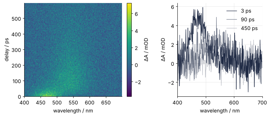
Two things are obvious. A band near 470 nm is strong at the earliest delays and fades within the first hundred picoseconds, while a band near 540 nm grows as it fades and lingers for hundreds of picoseconds. Over all of it lies noise, visible in every spectrum.
What is not obvious is how many species made this. By Beer-Lambert, absorbances add. A single species contributes its spectrum, scaled at every delay by how much of it is present: one spectrum shape times one time course, a matrix whose rows are all multiples of one spectrum. The rank of a matrix is the smallest number of such pieces that add up to it, so two species without noise give a matrix of rank 2, and the 60,000 numbers are really two spectra and two time courses. Noise breaks this: no two pieces add up to the measured matrix anymore, and it has full rank, 200.
So the question is: how many species does this matrix contain, read from the numbers alone, without a kinetic model and without being told how large the noise is? The answer comes at the end, as a count read off one plot, together with a cleaned matrix.
The idea: a matrix turns a circle into an ellipse
Put the 60,000 numbers aside and take a small matrix, \(M = \begin{bmatrix} 2 & 1 \\ 0 & 1 \end{bmatrix}\). Apply it to every vector of length 1, every point on the unit circle, and the points land on an ellipse. Every matrix does that: a circle goes in, an ellipse comes out. You may have met this ellipse in The condition number: how many digits a linear solve can lose, where its axes decided how many digits a solve loses. What is new here is that the ellipse hands you a factorization of the matrix itself.
Among all input directions there are two perpendicular ones, \(v_1\) and \(v_2\), that land exactly on the axes of the ellipse. Their images point along two perpendicular directions \(u_1\) and \(u_2\), and the half-axes have lengths \(\sigma_1\) and \(\sigma_2\), the singular values. So \(M\) can be carried out in three moves: turn the plane until \(v_1\) and \(v_2\) lie on the coordinate axes, stretch along the axes by \(\sigma_1\) and \(\sigma_2\), and turn again until the axes point along \(u_1\) and \(u_2\). A turn is a matrix with orthonormal columns, which changes no length (a rotation, or a reflection), and the stretch is a diagonal matrix. As a product, \(M = U\Sigma V^{\top}\).
Show code
M = np.array([[2.0, 1.0], [0.0, 1.0]])
U_M, s_M, Vt_M = np.linalg.svd(M)

print(f"singular values     {s_M[0]:.3f}, {s_M[1]:.3f}")
print(f"eigenvalues         {', '.join(f'{x:.3f}' for x in np.linalg.eigvals(M))}")
print(f"|det M|             {abs(np.linalg.det(M)):.3f}   product of singular values {s_M.prod():.3f}")
print(f"v1 at {np.degrees(np.arctan2(Vt_M[0, 1], Vt_M[0, 0])):.1f} deg, "
      f"u1 at {np.degrees(np.arctan2(U_M[1, 0], U_M[0, 0])):.1f} deg from the x axis")
print(f"U @ Sigma @ Vt == M: {np.allclose(U_M @ np.diag(s_M) @ Vt_M, M, rtol=0, atol=1e-15)}")

phi = np.linspace(0, 2 * np.pi, 200)
circle = np.vstack([np.cos(phi), np.sin(phi)])
marks = circle[:, ::25]                                # dots, so that a turn is visible
stages = [("circle", np.eye(2)), ("after Vᵀ", Vt_M), ("after Σ", np.diag(s_M) @ Vt_M),
          ("after U = M", U_M @ np.diag(s_M) @ Vt_M)]

fig, axes = plt.subplots(1, 4, figsize=(8, 2.0), sharex=True, sharey=True, layout="constrained")
for k, (ax, (label, A)) in enumerate(zip(axes, stages)):
    ax.plot(*(A @ circle), color=INK, lw=1.6)
    ax.plot(*(A @ marks), "o", color=INK, ms=3)
    for head, color in zip((A @ Vt_M.T).T, [ACCENT, SECOND]):   # where v1 and v2 have gone
        ax.annotate("", head, (0, 0), arrowprops=dict(arrowstyle="-|>", color=color, lw=1.6))
    ax.text(0.02, 0.98, label, transform=ax.transAxes, va="top")
    ax.set(aspect="equal", xlim=(-2.5, 2.5), ylim=(-1.6, 1.6), xticks=[-2, 0, 2], yticks=[-1, 0, 1])
axes[2].text(s_M[0] / 2, -0.5, f"{s_M[0]:.2f}", color=ACCENT, ha="center")
axes[2].text(0.15, s_M[1] + 0.12, f"{s_M[1]:.2f}", color=SECOND)
axes[0].set(xlabel="x", ylabel="y")
plt.show()
singular values     2.288, 0.874
eigenvalues         2.000, 1.000
|det M|             2.000   product of singular values 2.000
v1 at 31.7 deg, u1 at 13.3 deg from the x axis
U @ Sigma @ Vt == M: True
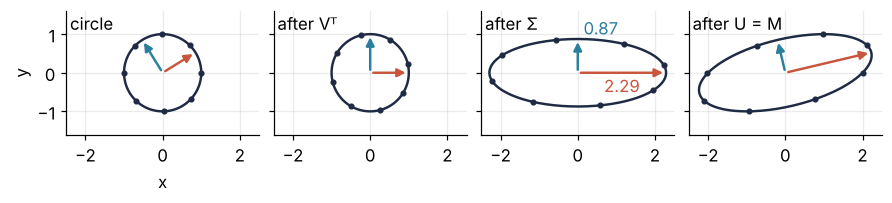
The cell finds \(\sigma_1 = 2.288\) and \(\sigma_2 = 0.874\), with \(v_1\) at 31.7° and \(u_1\) at 13.3° from the \(x\) axis, and the product of the three factors gives back \(M\) to machine precision. The singular values are not the eigenvalues, which for \(M\) are 2 and 1. The two coincide only for a symmetric matrix whose eigenvalues are not negative. Their product is \(|\det M| = 2\), the factor by which \(M\) scales areas.
Show code
"""Rotation, stretch, rotation: the unit circle mapped by M = [[2, 1], [0, 1]] in the three
factors of its singular value decomposition, M = U Σ Vᵀ.

Renders ../../assets/svd-circle.gif. Run it from any directory:

    python scene.py
"""
from pathlib import Path

import numpy as np
import matplotlib.pyplot as plt
from matplotlib.animation import FuncAnimation, PillowWriter
from PIL import Image

OUT = Path(__file__).resolve().parents[2] / "assets" / "svd-circle.gif"
INK, ACCENT, SECOND, MUTED = "#1f2a44", "#c8553d", "#2a7f9e", "#8a8f98"
plt.rcParams.update({"axes.spines.top": False, "axes.spines.right": False,
                     "axes.grid": True, "grid.alpha": 0.25, "font.size": 11})

# ---- the factorization, and the rotation angle of each orthogonal factor
M = np.array([[2.0, 1.0], [0.0, 1.0]])
U, s, Vt = np.linalg.svd(M)
angle_Vt = np.arctan2(Vt[1, 0], Vt[0, 0])             # both factors are proper rotations here
angle_U = np.arctan2(U[1, 0], U[0, 0])

def rotation(a):
    return np.array([[np.cos(a), -np.sin(a)], [np.sin(a), np.cos(a)]])

def matrix_at(stage, x):
    """The partial product after `stage` complete factors and a fraction x of the next one."""
    if stage == 0:
        return rotation(x * angle_Vt)
    if stage == 1:
        return np.diag(1 + x * (s - 1)) @ Vt
    return rotation(x * angle_U) @ np.diag(s) @ Vt

# ---- the frame schedule: three stages, a hold on M, the way back, a hold on the circle
# A frame is (stage, fraction of that stage done, True on the way back).
ease = lambda x: 0.5 - 0.5 * np.cos(np.pi * x)
forward = [(k, ease(x), False) for k in range(3) for x in np.linspace(0, 1, 24)]
back = [(k, x, True) for k, x, _ in forward[::-2]]
frames = [(0, 0.0, False)] * 8 + forward + [(2, 1.0, False)] * 14 + back + [(0, 0.0, False)] * 4
titles = [f"rotate by Vᵀ  ({np.degrees(angle_Vt):+.1f}°)",
          f"stretch by Σ  ({s[0]:.2f} and {s[1]:.2f} along the axes)",
          f"rotate by U  ({np.degrees(angle_U):+.1f}°)"]

phi = np.linspace(0, 2 * np.pi, 200)
circle = np.vstack([np.cos(phi), np.sin(phi)])
marks = circle[:, ::25]                                # eight dots, so that a rotation is visible
v = Vt.T                                               # columns v1, v2: the input directions

# ---- figure, drawn once
fig, ax = plt.subplots(figsize=(5.6, 2.8), dpi=100, layout="constrained")   # 560 x 280 px, text legible on a phone
ax.plot(*circle, color=MUTED, lw=1, ls="--")
ax.set(xlim=(-2.7, 2.7), ylim=(-1.35, 1.35), aspect="equal", xlabel="x", ylabel="y")
(shape,) = ax.plot([], [], color=INK, lw=1.8)
(dots,) = ax.plot([], [], "o", color=INK, ms=5)
arrows = [ax.annotate("", (0, 0), (0, 0), arrowprops=dict(arrowstyle="-|>", lw=2, color=color))
          for color in (ACCENT, SECOND)]                # v1 and its image red, v2 and its image teal
title = ax.set_title("", loc="left")

# ---- one frame: a function of the frame value alone
def update(frame):
    stage, x, returning = frame
    A = matrix_at(stage, x)
    shape.set_data(*(A @ circle))
    dots.set_data(*(A @ marks))
    done = (stage, x) == (2, 1.0) and not returning
    for arrow, head in zip(arrows, (A @ v).T):
        arrow.xy = head
    if stage == 0 and x == 0:
        title.set_text("the unit circle, with v₁ and v₂")
    elif done:
        title.set_text("U Σ Vᵀ = M: the arrows are σ₁u₁ and σ₂u₂")
    elif returning:
        title.set_text("back to the unit circle")
    else:
        title.set_text(titles[stage])

# ---- render, and read back what was written
OUT.parent.mkdir(exist_ok=True)
FuncAnimation(fig, update, frames=frames).save(OUT, writer=PillowWriter(fps=12))
plt.close(fig)
with Image.open(OUT) as im:                            # Pillow merges repeated frames into longer ones
    duration = 0
    for i in range(im.n_frames):
        im.seek(i)
        duration += im.info["duration"]
    print(f"{OUT.name}: {im.width} x {im.height} px, {len(frames)} frames, "
          f"{duration / 1000:.1f} s, {OUT.stat().st_size / 1024:,.0f} kB")
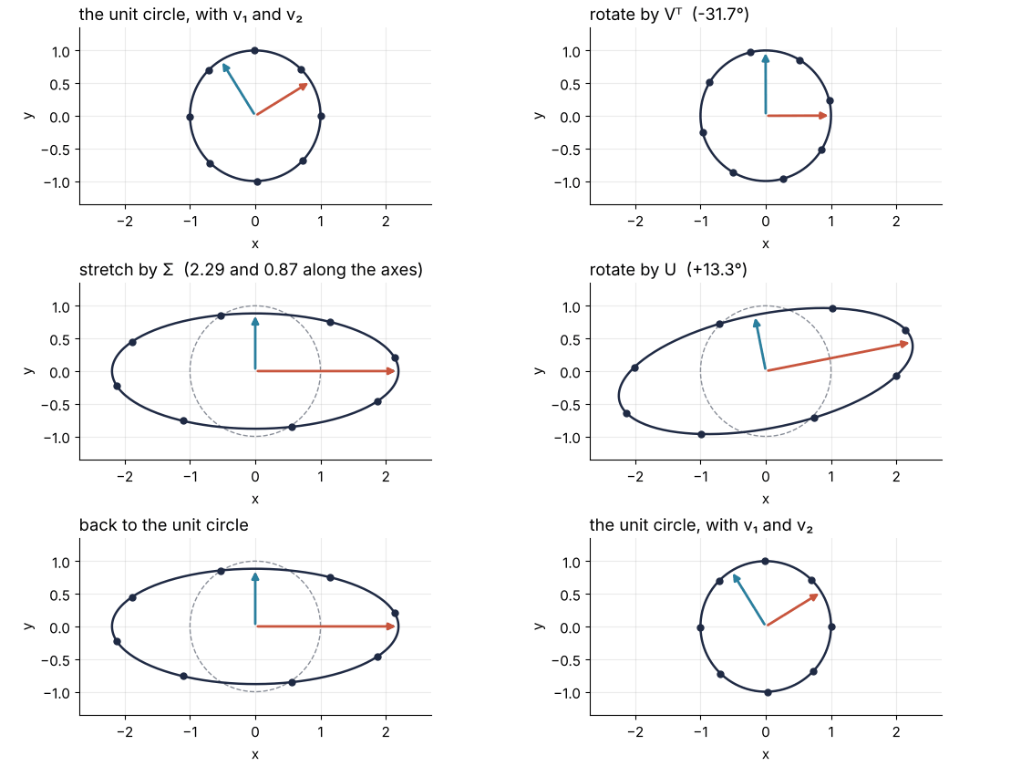
Watch the shape during the two turns: the dots slide around it, and its form does not change. All the stretching happens in the middle stage, along the coordinate axes.
The data matrix is not square, and the picture survives with one change. \(D\) takes a vector of 300 numbers, one per wavelength, and returns 200, one per delay, so you can call the input a spectrum and the output a time course, as long as you remember that this is geometry and not anything the spectrometer does. \(V^{\top}\) turns the 300-dimensional input space, \(\Sigma\) stretches along 200 axes and sends the remaining 100 input directions to zero, and \(U\) turns the result into the 200-dimensional output space. The unit sphere becomes an ellipsoid with at most 200 axes, and the singular values are their lengths. Nobody can draw it. The 2 × 2 picture is the one to keep in mind.
Layers ordered by size
The product \(U\Sigma V^{\top}\) can be multiplied out another way. Take \(\sigma_1\), the first column of \(U\), and the first row of \(V^{\top}\), and form \(\sigma_1 u_1 v_1^{\top}\), a column times a row. The result is a full matrix in which every row is a multiple of \(v_1^{\top}\), a matrix of rank one. Do the same for every \(i\) and add:
That this sum equals the product is ordinary matrix multiplication with the terms regrouped, and on \(M\) you can check it by eye:
Show code
layers_M = [s_M[i] * np.outer(U_M[:, i], Vt_M[i]) for i in range(2)]
for i, L in enumerate(layers_M, start=1):
    print(f"layer {i}:  [[{L[0, 0]:6.3f}, {L[0, 1]:6.3f}], [{L[1, 0]:6.3f}, {L[1, 1]:6.3f}]]")
total = layers_M[0] + layers_M[1]
print(f"sum:      [[{total[0, 0]:6.3f}, {total[0, 1]:6.3f}], [{total[1, 0]:6.3f}, {total[1, 1]:6.3f}]]")
layer 1:  [[ 1.894,  1.171], [ 0.447,  0.276]]
layer 2:  [[ 0.106, -0.171], [-0.447,  0.724]]
sum:      [[ 2.000,  1.000], [ 0.000,  1.000]]
Add the layers entry by entry, 1.894 + 0.106 = 2 in the top left and 0.447 − 0.447 = 0 in the bottom left, and you have \(M\) back. Each layer is what one axis of the ellipse contributes: the first sends \(v_1\) to \(\sigma_1 u_1\) and every vector perpendicular to \(v_1\) to zero.
Now take a layer of the data. \(\sigma_i u_i v_i^{\top}\) is one spectrum shape, \(v_i\), times one time course, \(u_i\), the same form a single species has. The SVD writes \(D\) as a sum of 200 such layers and orders them by size, because \(\sigma_1 \ge \sigma_2 \ge \dots\) Here are \(D\), its first two layers, and the other 198 added up, on one color scale, RdBu_r, red for positive and blue for negative:
Show code
U, s, Vt = np.linalg.svd(D, full_matrices=False)
sign = np.sign(Vt.sum(axis=1))                         # each pair (u_i, v_i) has a free sign; fix it so v_i sums positive
U, Vt = U * sign, Vt * sign[:, None]
layer = lambda i: s[i] * np.outer(U[:, i], Vt[i])
panels = [("D", D), (f"layer 1\nσ₁ = {s[0]:.1f}", layer(0)), (f"layer 2\nσ₂ = {s[1]:.1f}", layer(1)),
          ("layers 3\nto 200", D - layer(0) - layer(1))]

fig, axes = plt.subplots(1, 4, figsize=(8, 2.9), sharey=True, layout="constrained")
for ax, (label, img) in zip(axes, panels):
    im = ax.imshow(img, aspect="auto", origin="lower", extent=extent, cmap="RdBu_r", vmin=-5, vmax=5)
    ax.grid(False)
    ax.text(0, 1.02, label, transform=ax.transAxes, va="bottom", linespacing=1.1)
    ax.set(xticks=[450, 600])
axes[0].set(xlabel="wavelength / nm", ylabel="delay / ps")
fig.colorbar(im, ax=axes, label="ΔA / mOD", shrink=0.9)
plt.show()
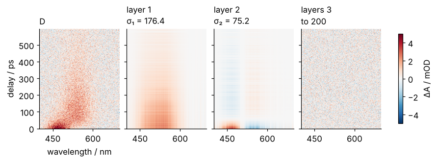
The first layer, with \(\sigma_1 = 176.4\), is one broad band that covers both species at once and fades slowly. The second, with \(\sigma_2 = 75.2\), is a correction with two signs: in the first 50 ps it adds absorbance near 470 nm and takes some away near 540 nm, and later it does the reverse, faintly. The remaining 198 layers together look like the noise and nothing else, and the largest of them has \(\sigma_3 = 30.9\). That leaves two questions: why is dropping the small layers the best thing to do, and where exactly does small begin?
Formalization
For any \(m \times n\) matrix \(A\), the singular value decomposition is
where \(U\) and \(V\) have orthonormal columns and \(\Sigma\) is diagonal with entries \(\sigma_1 \ge \sigma_2 \ge \dots \ge \sigma_r \ge 0\), the singular values, with \(r = \min(m, n)\). For \(D\), with \(m < n\), the reduced form that np.linalg.svd returns with full_matrices=False suffices: \(U\) and \(\Sigma\) are 200 × 200, and \(V^{\top}\) is 200 × 300 instead of 300 × 300. Distances between matrices are measured in the Frobenius norm \(\|A\|_F\), the square root of the sum of all squared entries.
The decomposition has three consequences you need every time you use it.
The best rank-k approximation. Keep the first \(k\) layers and call the result \(A_k\). The Eckart-Young theorem says that no matrix of rank \(k\) is closer to \(A\) in the Frobenius norm, and that the distance is set by what was dropped:
With \(k = 0\) the formula says \(\|A\|_F^2 = \sum_i \sigma_i^2\): the squared singular values share out the total of all squared entries, as the components share out the total variance in PCA with scikit-learn.
Show code
m, n = D.shape
rms = lambda X: np.sqrt(np.mean(X**2))
D2 = (U[:, :2] * s[:2]) @ Vt[:2]

print(f"sum of sigma^2       {np.sum(s**2):10.1f} mOD^2   sum of D^2 {np.sum(D**2):10.1f} mOD^2")
print(f"|D - D2|_F           {np.linalg.norm(D - D2):10.2f} mOD     root of dropped sigma^2 {np.sqrt(np.sum(s[2:]**2)):.2f} mOD")
print(f"rms of D - D_true    {rms(D - D_true):10.3f} mOD     of D2 - D_true {rms(D2 - D_true):.3f} mOD")
sum of sigma^2          96528.2 mOD^2   sum of D^2    96528.2 mOD^2
|D - D2|_F               244.44 mOD     root of dropped sigma^2 244.44 mOD
rms of D - D_true         1.007 mOD     of D2 - D_true 0.138 mOD
On \(D\) the identity holds at 96,528 mOD², and \(\|D - D_2\|_F\) is 244.44 mOD, the root of the dropped \(\sigma_i^2\). The rms error against the noise-free matrix falls from 1.007 mOD in \(D\) to 0.138 mOD in \(D_2\), and a rough count says why. White noise spreads its power evenly over all 60,000 directions in the space of 200 × 300 matrices.
Near \(D\), the rank-2 matrices form a surface, flat to a good approximation, with about 2 × (200 + 300) = 1,000 directions, one per number it takes to write down two time courses and two spectra. Truncation picks the nearest point on it, so it keeps the noise along those 1,000 directions and drops it along the other 59,000. That leaves a sixtieth of the noise power, \(\sqrt{1/60} \approx 0.13\) of its amplitude.
Singular values are roots of eigenvalues. Multiply \(A\) by its transpose and \(U\) drops out, because \(U^{\top}U\) is the identity: \(A^{\top}A = V\Sigma^2V^{\top}\), the eigendecomposition of a symmetric matrix. So the \(\sigma_i^2\) are the eigenvalues of \(A^{\top}A\) and the \(v_i\) its eigenvectors, which eigh computes. Still, call svd. The condition number is the ratio \(\sigma_1/\sigma_r\), and forming \(A^{\top}A\) squares it: a singular value \(10^{-9}\) times the largest becomes an eigenvalue \(10^{-18}\) times the largest, below the 16 digits a double holds.
Show code
print(f"svd                      {', '.join(f'{x:.4f}' for x in s[:3])}")
print(f"sqrt(eigvalsh(D.T @ D))  {', '.join(f'{x:.4f}' for x in np.sqrt(np.linalg.eigvalsh(D.T @ D)[::-1][:3]))}")
gen = np.random.default_rng(198)                       # a 5 x 5 test matrix with singular values 1 to 1e-9
Q1, _ = np.linalg.qr(gen.standard_normal((5, 5)))
Q2, _ = np.linalg.qr(gen.standard_normal((5, 5)))
A = Q1 @ np.diag([1, 1e-2, 1e-4, 1e-6, 1e-9]) @ Q2.T
print(f"5 x 5: smallest sigma by svd {np.linalg.svd(A, compute_uv=False)[-1]:.2e}, "
      f"smallest eigenvalue of A.T @ A {np.linalg.eigvalsh(A.T @ A)[0]:.2e} (should be 1.00e-18)")
svd                      176.3935, 75.2366, 30.9192
sqrt(eigvalsh(D.T @ D))  176.3935, 75.2366, 30.9192
5 x 5: smallest sigma by svd 1.00e-09, smallest eigenvalue of A.T @ A -1.60e-17 (should be 1.00e-18)
On \(D\) the two routes agree to all four printed decimals. On a 5 × 5 test matrix with singular values from 1 down to \(10^{-9}\), svd returns the smallest as 1.00 × 10⁻⁹, while eigvalsh returns its square as −1.60 × 10⁻¹⁷, which is not even positive.
The noise floor. A matrix of pure noise, \(m \times n\) independent entries of standard deviation \(\eta\) (\(\sigma\) is taken), has no structure, yet its singular values are not zero. They fill a band whose upper edge is close to \(\eta(\sqrt{m} + \sqrt{n})\), a consequence of the Marchenko-Pastur law for their squares, exact as \(m\) and \(n\) grow. On a real measurement nobody hands you \(\eta\), so take it from the data. Neighboring wavelengths 1 nm apart see almost the same absorbance but independent noise, so subtracting neighboring columns cancels the signal and leaves noise of variance \(2\eta^2\):
Show code
s_noise = np.linalg.svd(D - D_true, compute_uv=False)
print(f"noise alone: sigma from {s_noise[-1]:.2f} to {s_noise[0]:.2f}, "
      f"predicted {np.sqrt(n) - np.sqrt(m):.2f} to {np.sqrt(n) + np.sqrt(m):.2f}")
eta_hat = np.diff(D, axis=1).std() / np.sqrt(2)
edge = eta_hat * (np.sqrt(m) + np.sqrt(n))
print(f"eta_hat {eta_hat:.3f} mOD, edge {edge:.2f}, singular values above it: {np.sum(s > edge)}")
print(f"rms of neighbor differences: signal {rms(np.diff(D_true, axis=1)):.3f} mOD, "
      f"noise {rms(np.diff(D - D_true, axis=1)):.3f} mOD")

energy = np.cumsum(s**2) / np.sum(s**2)
print(f"\nshare of sum of sigma^2 in 2 components: {100 * energy[1]:.0f} %, "
      f"components for 95 %: {np.searchsorted(energy, 0.95) + 1}")
D5 = D_true + 5.0 * np.random.default_rng(198).standard_normal(D_true.shape)
s5 = np.linalg.svd(D5, compute_uv=False)
eta_hat5 = np.diff(D5, axis=1).std() / np.sqrt(2)
print(f"5 mOD noise: sigma_2 {s5[1]:.1f}, sigma_3 {s5[2]:.1f}, edge {5 * (np.sqrt(m) + np.sqrt(n)):.1f} "
      f"(true eta), {eta_hat5 * (np.sqrt(m) + np.sqrt(n)):.1f} (estimated)")
noise alone: sigma from 3.51 to 31.01, predicted 3.18 to 31.46
eta_hat 1.008 mOD, edge 31.72, singular values above it: 2
rms of neighbor differences: signal 0.013 mOD, noise 1.426 mOD

share of sum of sigma^2 in 2 components: 38 %, components for 95 %: 130
5 mOD noise: sigma_2 155.1, sigma_3 153.9, edge 157.3 (true eta), 158.6 (estimated)
For the noise of this example alone, \(\eta = 1\) mOD, the edge is at 31.46 and the singular values run from 3.51 to 31.01. For \(D\) the estimate gives \(\hat\eta = 1.008\) mOD, an edge at 31.72, and two singular values above it: the effective rank, the count above the floor, is 2. The estimate needs a signal that changes little from one grid point to the next (here 0.013 mOD rms between neighbors, against 1.426 mOD for the noise) and noise that is independent from point to point, which the edge formula assumes anyway. When probe fluctuations correlate the noise across wavelengths, the second condition fails, and the floor has to come from a record without signal, such as delays before time zero, which hold only noise.
The floor is also a detection limit: with 5 mOD of noise, \(\sigma_2 = 155.1\) falls below the edge, 157.3 with the true \(\eta\) and 158.6 estimated, and sits next to \(\sigma_3 = 153.9\). And it is why a percentage rule fails: the two real components hold only 38 % of \(\sum_i \sigma_i^2\), and keeping 95 % would take 130 components, most of them noise. This is the PCA tutorial's elbow rule, with an elbow you can compute.
See it in code
The whole procedure, as you would run it on your own matrix, uses nothing the simulation knows, except in the one line that compares with the noise-free matrix:
Show code
U, s, Vt = np.linalg.svd(D, full_matrices=False)
sign = np.sign(Vt.sum(axis=1))                         # the sign of each pair is free; make each v_i sum positive
U, Vt = U * sign, Vt * sign[:, None]

m, n = D.shape
eta_hat = np.diff(D, axis=1).std() / np.sqrt(2)        # neighboring wavelengths: same signal, independent noise
edge = eta_hat * (np.sqrt(m) + np.sqrt(n))
rank = int(np.sum(s > edge))
D_k = (U[:, :rank] * s[:rank]) @ Vt[:rank]

print(f"U {U.shape}, s {s.shape}, Vt {Vt.shape}")
print(f"first six singular values: {', '.join(f'{x:.1f}' for x in s[:6])}")
print(f"eta_hat = {eta_hat:.3f} mOD, edge = {edge:.2f}, rank = {rank}")
print(f"rms of D - D_k = {rms(D - D_k):.2f} mOD (should match eta_hat)")
print(f"rms against the noise-free matrix: {rms(D - D_true):.2f} mOD before, {rms(D_k - D_true):.2f} mOD after")
i470, i540 = np.searchsorted(wl, [470, 540])
print(f"v2 at 470 nm {Vt[1, i470]:+.3f}, at 540 nm {Vt[1, i540]:+.3f}")

fig, axes = plt.subplots(2, 2, figsize=(8, 6), layout="constrained")
ax = axes[0, 0]
ax.semilogy(np.arange(rank + 1, m + 1), s[rank:], "o", color=INK, ms=3)
for i, color in enumerate([ACCENT, SECOND][:rank]):    # component 1 red, component 2 teal, as in every panel
    ax.semilogy(i + 1, s[i], "o", color=color, ms=6)
ax.axhline(edge, color=MUTED, ls="--", lw=1)
ax.text(m, edge * 1.15, f"noise edge {edge:.1f}", color=MUTED, ha="right", va="bottom")
ax.text(12, np.sqrt(s[0] * s[1]), f"rank {rank}", color=INK, va="center")   # between the two dots
ax.set(xlabel="index i", ylabel="σᵢ / mOD")
ax = axes[0, 1]
for i, color in enumerate([ACCENT, SECOND]):
    ax.plot(t, U[:, i], color=color)
ax.text(300, 0.095, "u₁", color=ACCENT, ha="center", va="bottom")
ax.text(30, 0.32, "u₂", color=SECOND, ha="left", va="center")
ax.set(xlabel="delay / ps", ylabel="uᵢ / dimensionless")
ax = axes[1, 0]
for spec, name in [(s_A, "A"), (s_B, "B")]:
    unit = spec / np.linalg.norm(spec)                 # true spectra, scaled like the unit vectors v_i
    ax.plot(wl, unit, color=MUTED, lw=1)
    ax.text(wl[np.argmax(unit)], 0.17 if name == "A" else unit.max() + 0.012, name,
            color=MUTED, ha="center", va="bottom")
for i, color in enumerate([ACCENT, SECOND]):
    ax.plot(wl, Vt[i], color=color)
ax.text(640, 0.055, "v₁", color=ACCENT, ha="left", va="bottom")
ax.text(495, -0.07, "v₂", color=SECOND, ha="right", va="center")
ax.axhline(0, color=MUTED, lw=0.8)
ax.set(xlabel="wavelength / nm", ylabel="vᵢ / dimensionless", ylim=(-0.12, 0.2))
ax = axes[1, 1]
im = ax.imshow(D - D_k, aspect="auto", origin="lower", extent=extent, cmap="RdBu_r", vmin=-3, vmax=3)
ax.grid(False)
fig.colorbar(im, ax=ax, label="residual / mOD")
ax.set(xlabel="wavelength / nm", ylabel="delay / ps")
plt.show()
U (200, 200), s (200,), Vt (200, 300)
first six singular values: 176.4, 75.2, 30.9, 30.6, 29.9, 29.8
eta_hat = 1.008 mOD, edge = 31.72, rank = 2
rms of D - D_k = 1.00 mOD (should match eta_hat)
rms against the noise-free matrix: 1.01 mOD before, 0.14 mOD after
v2 at 470 nm +0.115, at 540 nm -0.063
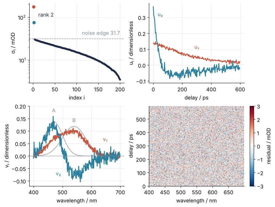
The procedure lands on the count from the noise floor, rank 2. The rms of what truncation removed, 1.00 mOD, matches \(\hat\eta\): a check you can run on real data too, though not a way to find \(\hat\eta\). Only the comparison with the noise-free matrix needs the simulation: 1.01 mOD before truncation and 0.14 mOD after, as in the formalization. Two species went into the simulation, and two singular values came out above a floor the data set for itself. The residual in the last panel is noise without structure.
Each pair \(u_i\), \(v_i\) is defined only up to a common sign, since flipping both leaves \(\sigma_i u_i v_i^{\top}\) unchanged, and the cell flips each pair so that \(v_i\) sums positive. Under that choice \(v_2\) is positive under the 470 nm band and negative under the 540 nm band, a shape no absorption spectrum in this model has, and the other sign only turns it upside down. So \(v_1\) and \(v_2\) are not the spectra of A and B. Any mixture of them, with the matching mixture of \(u_1\) and \(u_2\), fits the data equally well, and picking the physical one takes a kinetic model, global or target analysis. What the SVD gives you is the number of species and the two-dimensional space their spectra live in.
Where it shows up
The pump-probe matrix is one case of a pattern that runs through science: many measurements of a few underlying things, arranged as a table, and the question of how many things there are.
- Chemistry and biology: principal component analysis. PCA is the SVD of the data matrix after each column's mean is subtracted: the scores are \(U\Sigma\), the loadings are \(V\), and the explained variance ratio is \(\sigma_i^2 / \sum_j \sigma_j^2\). PCA with scikit-learn reduced sixty UV-Vis spectra to two dimensions that way, after also scaling each column.
- Geology and climate science: empirical orthogonal functions. Climate scientists arrange sea-surface temperature anomalies as a matrix of months by grid points and take its SVD, the spatial patterns in \(V\) and their time series in \(U\). The leading pattern in the tropical Pacific is El Niño.
- Physics and engineering: least squares and the pseudoinverse. For an overdetermined or rank-deficient system \(Ax \approx b\), the least-squares solution of smallest length is \(x = V\Sigma^{+}U^{\top}b\), with \(\Sigma^{+}\) inverting the nonzero \(\sigma_i\);
np.linalg.pinvcomputes it from the SVD, andnp.linalg.lstsqdrops small singular values below itsrcondcutoff (Least squares: what a fit minimizes, and why the residuals are squared). Dropping the tiny \(\sigma_i\) on purpose is truncated-SVD regularization, the first thing to try on an ill-posed inverse problem. - Image processing: compression. A grayscale image is a matrix of pixel values, and keeping \(k\) layers stores \(k(m + n + 1)\) numbers instead of \(mn\). A 1000 × 1000 image at \(k = 50\) needs 100,050 numbers instead of a million.
- Data science: recommender systems. A matrix of users by items, filled with ratings, is close to low rank because tastes come in a few kinds. Low-rank factorizations of that matrix were at the center of the methods that competed for the Netflix Prize.
- Quantum physics: the Schmidt decomposition. The coefficients of a state of two subsystems form a matrix, and its SVD is the Schmidt decomposition. More than one nonzero singular value means the two parts are entangled.
In every case the same reading carries over: large singular values are structure, the flat floor is noise, and the count above the floor is the number of independent things the data can tell apart.
Further reading
numpy.linalg.svdforfull_matrices, and the order of the singular values;scipy.linalg.svdfor the choice of LAPACK driver.- Trefethen and Bau, Numerical Linear Algebra, lectures 4 and 5, for the SVD, its geometry, and the best low-rank approximation. Strang, Linear Algebra and Learning from Data, for the data side.
- Gavish and Donoho, "The optimal hard threshold for singular values is 4/√3", IEEE Transactions on Information Theory (2014), for a threshold from the median singular value, when the signal is not smooth on the grid or the noise cannot be estimated from differences.
- van Stokkum, Larsen, and van Grondelle, "Global and target analysis of time-resolved spectra", Biochimica et Biophysica Acta (2004), for turning the singular vectors into species spectra with a kinetic model.
- Related tutorials on this site: The condition number: how many digits a linear solve can lose; Eigenvalues with numpy.linalg: normal modes of coupled oscillators; PCA with scikit-learn: sixty absorption spectra in two dimensions; Least squares: what a fit minimizes, and why the residuals are squared; Rotations with scipy.spatial.transform: superpose two conformers, where the SVD finds the best rotation; Matplotlib animation with FuncAnimation: a probe sweep as a small GIF, for how animations like the one above are built; planned: The singular value decomposition in Julia.
- Download the notebook. It was executed with the library versions in the header.