The condition number: how many digits a linear solve can lose

The question

Two straight lines, x + y = 2 and x + 1.001y = 2.001, cross at the point (1, 1). Change the second right-hand side by a thousandth, from 2.001 to 2.002, and ask np.linalg.solve for the crossing again:

Show code

Copy

import warnings

import numpy as np
import scipy.linalg
import matplotlib.pyplot as plt

plt.rcParams.update({
    "figure.figsize": (7, 3.6), "figure.dpi": 110,
    "axes.spines.top": False, "axes.spines.right": False,
    "axes.grid": True, "grid.alpha": 0.25,
    "font.size": 11, "lines.linewidth": 1.8,
})
INK, ACCENT, SECOND, MUTED = "#1f2a44", "#c8553d", "#2a7f9e", "#8a8f98"

eps = np.finfo(float).eps
norm = np.linalg.norm
A = np.array([[1, 1], [1, 1.001]])
b = np.array([2, 2.001])


def digits(x_hat, x_true):
    """Correct digits: minus log10 of the relative error in the 2-norm."""
    return -np.log10(norm(x_hat - x_true) / norm(x_true))


def angle(t):
    """Angle in degrees between x + y = 2 and x + (1 + t)y = 2 + t."""
    return np.degrees(np.arctan(1) - np.arctan(1 / (1 + t)))


x = np.linalg.solve(A, b)
b2 = np.array([2, 2.002])
x2 = np.linalg.solve(A, b2)
print(f"b = {b},  x = {x}")
print(f"b = {b2},  x = {x2}")
print(f"relative change of b: {100 * norm(b2 - b) / norm(b):.3f} %,  of x: {100 * norm(x2 - x) / norm(x):.0f} %")
print(f"angle between the lines: {angle(0.001):.4f}°")

xs = np.array([-0.5, 2.5])
fig, ax = plt.subplots(figsize=(7, 3.6))
ax.plot(xs, 2 - xs, color=INK, lw=3)
ax.plot(xs, (2.001 - xs) / 1.001, color=SECOND, lw=2)
ax.plot(xs, (2.002 - xs) / 1.001, color=ACCENT, lw=1)
ax.text(-0.4, 0.25, "x + y = 2", color=INK, ha="left")
ax.text(-0.4, -0.05, "x + 1.001y = 2.001", color=SECOND, ha="left")
ax.text(-0.4, -0.35, "x + 1.001y = 2.002", color=ACCENT, ha="left")
ax.plot(*x, "o", color=INK, ms=7, zorder=3)
ax.plot(*x2, "o", color=ACCENT, ms=7, zorder=3)
ax.annotate("(1, 1)", x, xytext=(10, 4), textcoords="offset points", color=INK)
ax.annotate("(0, 2) after the nudge", x2, xytext=(12, 8), textcoords="offset points", color=ACCENT)
ax.set(xlabel="x", ylabel="y", xlim=(-0.5, 2.5), ylim=(-0.5, 2.5), aspect="equal")
plt.show()

b = [2.    2.001],  x = [1. 1.]
b = [2.    2.002],  x = [0. 2.]
relative change of b: 0.035 %,  of x: 100 %
angle between the lines: 0.0286°

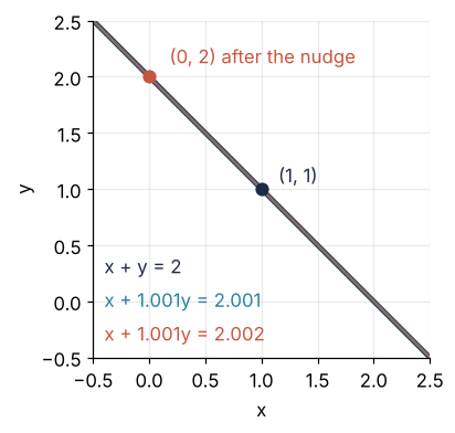
The first solve returns (1, 1), the second (0, 2). A change of 0.035 % in the data has moved the answer by 100 %, and how large such a jump can get is fixed by one number of the matrix, its condition number. In the picture the three lines lie on top of each other, the first one included, and only the two dots tell the systems apart.

The obvious culprit is the angle, and it is the right one as far as it goes. The lines meet at 0.0286°, and anyone who has tried to mark the crossing of two nearly parallel lines with a ruler knows that the point is poorly defined.

The less obvious part is how far this reaches. Every number in a computer already carries a change of about one part in 10¹⁶, the rounding described in Floating-point numbers, so every linear solve starts from nudged data. How much can a solve amplify a change in its data, and can you read that factor off the matrix before you solve? The condition number answers both, and it will be put to a test at the end: the 12 × 12 Hilbert matrix, whose entries all lie between 1/23 and 1 and look entirely harmless. Of the 16 digits a float carries, how many does a solve with it keep?

The idea: nearly parallel lines cross at a poorly defined point

Each equation of a 2 × 2 system is a line in the plane, and the solution is the point where the two lines cross. Changing a right-hand side shifts its line sideways, parallel to itself, and the crossing has to follow. When the lines meet at a steep angle, the crossing moves by about as much as the line did. When they meet at a shallow angle, the crossing slides along the other line, and the shallower the angle, the farther it slides.

To make that exact, tilt the second line by a parameter t. The lines x + y = 2 and x + (1 + t)y = 2 + t cross at (1, 1) for every t, and t = 0.001 is the system from the question. Nudge the second right-hand side by δ and the crossing moves to (1 − δ/t, 1 + δ/t), a distance of √2·δ/t. How far the crossing moves per unit of nudge is then √2/t, and it grows without limit as the tilt shrinks. Here are three tilts with the same nudge, δ = 0.001:

Show code

Copy

delta = 1e-3
fig, axes = plt.subplots(1, 3, figsize=(8, 3), sharey=True)
for ax, t in zip(axes, [1, 0.1, 0.001]):
    At = np.array([[1, 1], [1, 1 + t]])
    p0 = np.linalg.solve(At, [2, 2 + t])
    p1 = np.linalg.solve(At, [2, 2 + t + delta])
    shift = norm(p1 - p0)
    ax.plot(xs, 2 - xs, color=INK, lw=3)
    ax.plot(xs, (2 + t - xs) / (1 + t), color=SECOND, lw=2)
    ax.plot(xs, (2 + t + delta - xs) / (1 + t), color=ACCENT, lw=1)
    ax.plot(*p0, "o", color=INK, ms=6, zorder=3)
    ax.plot(*p1, "o", color=ACCENT, ms=6, zorder=3)
    ax.text(0.97, 0.97, f"t = {t:g}\nangle {angle(t):.1f}°\nshift {shift:.3g}" if t > 0.01 else
            f"t = {t:g}\nangle {angle(t):.2g}°\nshift {shift:.3g}",
            transform=ax.transAxes, ha="right", va="top")
    ax.set(xlabel="x", xlim=(-0.5, 2.5), ylim=(-0.5, 2.5), aspect="equal")
axes[0].set_ylabel("y")
plt.show()

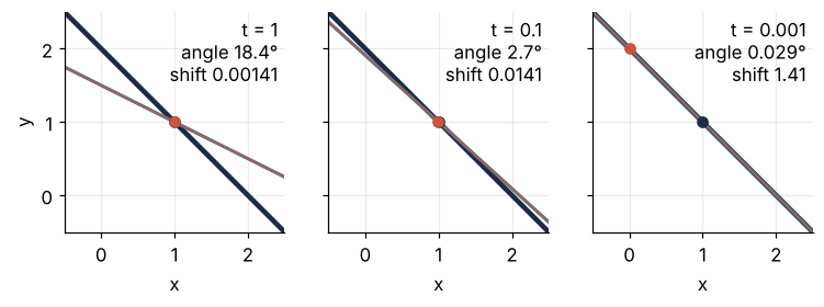
At t = 1 the lines meet at 18.4°, and the crossing moves by 0.00141, too little to see. At t = 0.1 the angle is 2.7° and the shift 0.0141. At t = 0.001 the angle is 0.029°, and the crossing has run 1.41 along the first line to (0, 2). Each factor of ten in the tilt is a factor of ten in the shift, while the nudge stayed the same.

Now let the tilt fall continuously from t = 1 to t = 0.001. The nudge stays at 0.001 throughout, so the last frame is the example from the question:

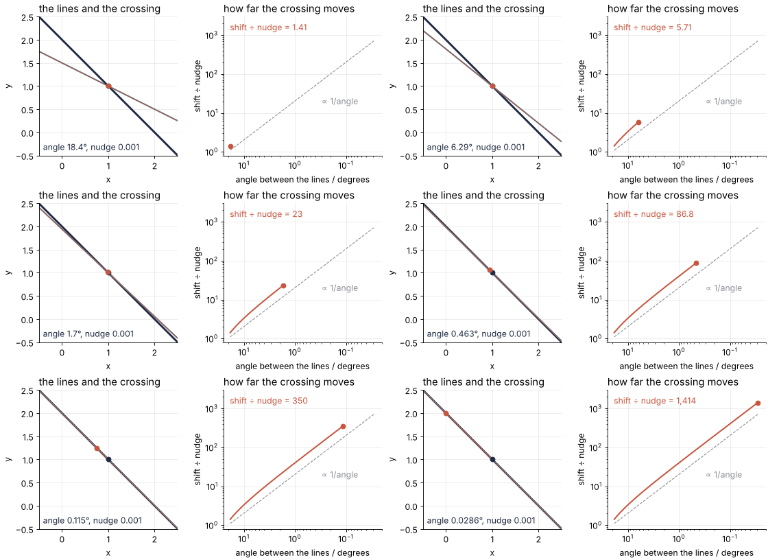
How I built this: Matplotlib animation with FuncAnimation: a probe sweep as a small GIF.

The right panel shows what the three snapshots cannot. The shift per unit of nudge rises smoothly from 1.41 at 18.4° to 1414 at 0.029°, and once the angle is below a few degrees it runs parallel to the dashed line of slope −1: halve the angle and you double the shift. Nowhere along the way does a system turn from good to bad. There is only a factor, and it grows.

A millionth in b, and how far x moves

Nudges by hand are not the only changes a right-hand side meets. Measured data carry errors, and every stored number is rounded. To compare such changes across problems, make the ratio from the animation relative: divide the relative change of x by the relative change of b, with ‖·‖ the ordinary length of a vector,

Relative changes do not depend on the units of x and b. The animation's last frame, b = (2, 2.001) nudged by (0, 0.001), has an amplification of 2829, twice the animation's 1414, because making both changes relative multiplies by ‖b‖/‖x‖ = 2.0. One direction of nudge says little about the others, though, so perturb b by a relative 10⁻⁶ in 1,000 random directions and measure each:

Show code

Copy

nudge = np.array([0, 0.001])
amp_nudge = (norm(np.linalg.solve(A, b + nudge) - x) / norm(x)) / (norm(nudge) / norm(b))
print(f"animation's nudge (0, 0.001):  amplification {amp_nudge:.0f},  ‖b‖/‖x‖ = {norm(b) / norm(x):.4f}")

rng = np.random.default_rng(1)
db = rng.standard_normal((1000, 2))
db *= (1e-6 * norm(b) / norm(db, axis=1))[:, None]          # every perturbation a relative 1e-6
dx = np.linalg.solve(A, (b + db).T).T - x
rel_b, rel_x = norm(db, axis=1) / norm(b), norm(dx, axis=1) / norm(x)
amp = rel_x / rel_b
print(f"1,000 random directions:       max {amp.max():.1f}, mean {amp.mean():.0f}, median {np.median(amp):.0f}")
for name, i in [("worst", amp.argmax()), ("mildest", amp.argmin())]:
    u = db[i] / norm(db[i])
    print(f"{name:8s} direction ({u[0]:+.3f}, {u[1]:+.3f}):  amplification {amp[i]:6.1f}, "
          f"x moves by a relative {rel_x[i]:.1e}")

i = amp.argmax()
fig, (ax1, ax2) = plt.subplots(1, 2, figsize=(7, 3.4))
sb, sx = 1e-6 * norm(b), 1e-3 * norm(x)
ax1.plot(db[:, 0] / sb, db[:, 1] / sb, "o", color=INK, ms=2, alpha=0.5)
ax1.plot(db[i, 0] / sb, db[i, 1] / sb, "o", color=ACCENT, ms=7)
ax1.set(xlabel="δb₁ / (10⁻⁶ ‖b‖)", ylabel="δb₂ / (10⁻⁶ ‖b‖)", xlim=(-1.5, 1.5), ylim=(-1.5, 1.5), aspect="equal")
ax2.plot([-5, 5], [5, -5], color=MUTED, lw=1, ls="--")
ax1.annotate("worst", (db[i, 0] / sb, db[i, 1] / sb), xytext=(8, -12), textcoords="offset points", color=ACCENT)
ax2.plot(dx[:, 0] / sx, dx[:, 1] / sx, "o", color=ACCENT, ms=2, alpha=0.5)
ax2.plot(dx[i, 0] / sx, dx[i, 1] / sx, "o", color=ACCENT, ms=7)
ax2.annotate("worst", (dx[i, 0] / sx, dx[i, 1] / sx), xytext=(-8, -6), textcoords="offset points",
             ha="right", va="top", color=ACCENT)
ax2.annotate("direction (1, −1)", (-3.6, 3.6), xytext=(3, 3), textcoords="offset points", rotation=-45,
             rotation_mode="anchor", ha="left", va="bottom", color=MUTED)
ax2.text(0.97, 0.97, f"max amplification {amp.max():.0f}", transform=ax2.transAxes, ha="right", va="top", color=ACCENT)
ax2.set(xlabel="δx₁ / (10⁻³ ‖x‖)", ylabel="δx₂ / (10⁻³ ‖x‖)", xlim=(-4, 4), ylim=(-4, 4), aspect="equal")
plt.tight_layout()
plt.show()

animation's nudge (0, 0.001):  amplification 2829,  ‖b‖/‖x‖ = 2.0005
1,000 random directions:       max 4002.0, mean 2585, median 2878
worst    direction (+0.707, -0.707):  amplification 4002.0, x moves by a relative 4.0e-03
mildest  direction (+0.704, +0.710):  amplification   18.0, x moves by a relative 1.8e-05

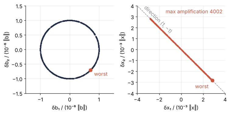
None of the 1,000 directions amplifies by more than 4002.0, and the mean is 2585. The worst sample points along (0.707, −0.707), the direction (1, −1), and moves x by a relative 4.0 × 10⁻³, which is 4002 times 10⁻⁶. The mildest points along (1, 1) and amplifies by only 18. On the left, b moved by the same amount in every direction. On the right, x moved along one line only, the direction of the first line, and the other direction barely registers.

A change in the sixth digit of b has reached the third digit of x. Digits are counted by the logarithm of the factor, so the loss is log10 4002 = 3.6 digits, not the 6 − 3 = 3 that the positions suggest. That leaves the question of where 4002 and the direction (1, −1) come from, and whether you can get them without trying directions.

Formalization

The length ‖x‖ of a vector is the Euclidean norm used above. A matrix gets a norm too: ‖A‖ is the largest factor by which A stretches any vector, the maximum of ‖Ax‖/‖x‖. Picture what A does to the circle of unit vectors. It turns the circle into an ellipse, whose half-axes are the singular values of A, σ_max and σ_min. So ‖A‖ = σ_max, and ‖A⁻¹‖ = 1/σ_min: A⁻¹ undoes A, so it stretches the short half-axis of the ellipse, of length σ_min, back to a unit vector, and no vector of the plane by more. For the example, σ_max = 2.0005 and σ_min = 4.999 × 10⁻⁴, with the long axis of the ellipse along (1, 1) and the short one along (1, −1): the two directions the samples found by trial.

U, sigma, Vt = np.linalg.svd(A)
print(f"singular values:          {sigma[0]:.4f} and {sigma[1]:.3e}")
print(f"long axis u_max           ({abs(U[0, 0]):.3f}, {abs(U[1, 0]):.3f})")
print(f"short axis                ({abs(U[0, 1]):.3f}, {-abs(U[1, 1]):.3f})")
print(f"‖A‖ = {norm(A, 2):.4f},  ‖A⁻¹‖ = {norm(np.linalg.inv(A), 2):.1f}")
print(f"κ(A) = {np.linalg.cond(A):.1f},  log10 κ = {np.log10(np.linalg.cond(A)):.2f}")
print(f"b along u_max:            |u_maxᵀ b| / ‖b‖ = {abs(U[:, 0] @ b) / norm(b):.6f}")
print(f"eps = {eps:.2g},  κ eps = {np.linalg.cond(A) * eps:.2g},  digits kept about {-np.log10(np.linalg.cond(A) * eps):.1f}")
print(f"det(A) = {np.linalg.det(A):.3g}")
S = 1e-3 * np.eye(10)
print(f"0.001 I₁₀: det = {np.linalg.det(S):.3g},  κ = {np.linalg.cond(S):.1f}")

singular values:          2.0005 and 4.999e-04
long axis u_max           (0.707, 0.707)
short axis                (0.707, -0.707)
‖A‖ = 2.0005,  ‖A⁻¹‖ = 2000.5
κ(A) = 4002.0,  log10 κ = 3.60
b along u_max:            |u_maxᵀ b| / ‖b‖ = 1.000000
eps = 2.2e-16,  κ eps = 8.9e-13,  digits kept about 12.1
det(A) = 0.001
0.001 I₁₀: det = 1e-30,  κ = 1.0

The condition number is the product of the two norms, which is the ratio of the longest half-axis to the shortest:

For the example, 2.0005 × 2000.5 = 4002. The identity matrix has κ = 1, no matrix has less, and a singular matrix, whose ellipse is flattened to a segment, has κ = ∞.

The bound takes three lines. Subtract Ax = b from A(x + δx) = b + δb to get A δx = δb, so δx = A⁻¹δb and ‖δx‖ ≤ ‖A⁻¹‖‖δb‖. From b = Ax follows ‖b‖ ≤ ‖A‖‖x‖. Divide the first inequality by ‖x‖ and use the second:

The bound is reached when both inequalities are equalities. The first one is an equality when δb points along the short axis of the ellipse, the direction A⁻¹ stretches most. The second is one when b points along the long axis, which the output calls u_max, the direction A stretches most. In the example b lies along u_max to six decimals, and the worst sample pointed along the short axis, which is why it reached 4002.

The bound is about changes in the data, but the solver rounds too. np.linalg.solve calls LAPACK's LU factorization with row exchanges, and each of its thousands of roundings is a relative error of about ε = 2.2 × 10⁻¹⁶. Following them through to x one by one is hopeless, so numerical analysis turns the question around: which data does the computed x̂ solve exactly? For LU with row exchanges the answer, called backward error analysis, is in practice a matrix A + δA whose entries differ from yours by a few ε relative. A nudge of A acts like one of b: subtracting Ax = b from (A + δA)x̂ = b gives A(x̂ − x) = −δA x̂, the old equation with δb = −δA x̂, so ‖x̂ − x‖/‖x‖ ≤ κ‖δA‖/‖A‖ to first order.

Three consequences follow, and you need them every time you solve.

Digits lost, log10 κ. A float carries a relative error of about ε before any solve, and the solver adds a few ε more, all of it a nudge of the data. The relative error of x is therefore about κε, and the digits kept are about −log10(κε) ≈ 16 − log10 κ. For the example that means 3.6 digits lost and about 12 kept. With measured data the 16 becomes the number of digits the data carries: data good to four digits, through κ = 100, leaves about two.

A bound, not a forecast. The random directions amplified by 2585 on average, not 4002, because a random δb rarely points along the short axis. A real solve usually loses fewer than log10 κ digits and never many more.

The determinant does not measure it. The example's determinant is 0.001, which looks like a warning. But 0.001 times the 10 × 10 identity has a determinant of 10⁻³⁰ and κ = 1.0, the best a matrix can have. Scaling a matrix changes its determinant by any factor you like and leaves κ alone.

See it in code

The Hilbert matrix Hₙ has the entries 1/(i + j − 1), and scipy.linalg.hilbert builds it. For n = 2 to 12 the cell takes the true solution x = (1, …, 1), computes b = Hₙx, solves with np.linalg.solve, and compares the digits kept with the rule of thumb 16 − log10 κ. At n = 12 it also tries scipy.linalg.solve:

Show code

Copy

ns = np.arange(2, 13)
kappa, kept = [], []
print(" n         κ   digits kept   16 − log10 κ")
for n in ns:
    H = scipy.linalg.hilbert(n)
    x_true = np.ones(n)
    b_n = H @ x_true
    kappa.append(np.linalg.cond(H))
    kept.append(digits(np.linalg.solve(H, b_n), x_true))
    print(f"{n:2d}  {kappa[-1]:9.3g}   {kept[-1]:11.2f}   {16 - np.log10(kappa[-1]):12.2f}")
kappa, kept = np.array(kappa), np.array(kept)
rule = 16 - np.log10(kappa)
print(f"\nper step of n: digits kept fall by {(kept[0] - kept[-1]) / 10:.2f}, log10 κ rises by {(rule[0] - rule[-1]) / 10:.2f}")
print(f"digits kept minus rule of thumb: from {(kept - rule).min():.2f} to {(kept - rule).max():.2f}")
print(f"entries of H₁₂ between {H.min():.4f} (1/23 = {1 / 23:.4f}) and {H.max():.0f}")
x_hat = np.linalg.solve(H, b_n)
print(f"n = 12: ‖x̂ − x‖/‖x‖ = {norm(x_hat - x_true) / norm(x_true):.2f},  ‖b − Hx̂‖/‖b‖ = {norm(b_n - H @ x_hat) / norm(b_n):.2g}")

with warnings.catch_warnings(record=True) as caught:      # print the warning, so both runs show the same text
    warnings.simplefilter("always")
    scipy.linalg.solve(H, b_n)
for w in caught:
    print(f"\nscipy.linalg.solve: {w.category.__name__}: {w.message}")
kappa1 = np.linalg.cond(H, 1)
print(f"κ₁(H₁₂) = {kappa1:.3g},  1/κ₁ = {1 / kappa1:.2g},  1/κ₂ = {1 / kappa[-1]:.2g},  κ₁/κ₂ = {kappa1 / kappa[-1]:.2f}")

fig, ax = plt.subplots(figsize=(7, 3.6))
ax.axhline(16, color=MUTED, lw=1, ls="--")
ax.plot(ns, rule, color=SECOND, lw=1.2)
ax.plot(ns, kept, "o-", color=ACCENT, lw=1.6, ms=6)
ax.text(2.2, 16.3, "16 digits of a float", color=MUTED, va="bottom")
ax.text(5.0, 9.0, "16 − log10 κ", color=SECOND, ha="right", va="top")
ax.annotate(f"{kept[-1]:.1f} digits kept", (12, kept[-1]), xytext=(12, 5.5), ha="right", color=ACCENT,
            arrowprops=dict(arrowstyle="-", color=ACCENT, lw=0.8, shrinkB=5))
ax.set(xlabel="Hilbert matrix size n", ylabel="correct digits", xlim=(1.7, 12.3), ylim=(-1, 17.5), yticks=[0, 4, 8, 12, 16])
plt.show()

 n         κ   digits kept   16 − log10 κ
 2       19.3         15.25          14.71
 3        524         14.08          13.28
 4   1.55e+04         13.47          11.81
 5   4.77e+05         11.90          10.32
 6    1.5e+07         10.39           8.83
 7   4.75e+08          8.75           7.32
 8   1.53e+10          7.17           5.82
 9   4.93e+11          5.52           4.31
10    1.6e+13          4.90           2.80
11   5.23e+14          2.95           1.28
12   1.62e+16          0.89          -0.21

per step of n: digits kept fall by 1.44, log10 κ rises by 1.49
digits kept minus rule of thumb: from 0.53 to 2.11
entries of H₁₂ between 0.0435 (1/23 = 0.0435) and 1
n = 12: ‖x̂ − x‖/‖x‖ = 0.13,  ‖b − Hx̂‖/‖b‖ = 1.1e-16

scipy.linalg.solve: LinAlgWarning: An ill-conditioned matrix detected: slice 0 has rcond = 2.5608932612789403e-17.
κ₁(H₁₂) = 3.99e+16,  1/κ₁ = 2.5e-17,  1/κ₂ = 6.2e-17,  κ₁/κ₂ = 2.46

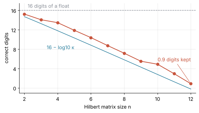
The kept digits fall by about 1.4 per step of n while log10 κ rises by about 1.5. They never fall below the rule of thumb and beat it by at most 2.1 digits, at n = 10; the last decimal of each count depends on the LAPACK build behind your NumPy. At n = 12 the solve keeps 0.9 digits, yet H₁₂x̂ reproduces b to a relative 1.1 × 10⁻¹⁶, as backward error analysis promised. The solver did its part: a matrix with every entry between 1/23 and 1 has taken 15 of 16 digits.

np.linalg.solve stays silent at every n. scipy.linalg.solve warns at n = 12 with rcond = 2.56 × 10⁻¹⁷, a cheap LAPACK estimate of 1/κ in the 1-norm, where ‖A‖₁ is the largest column sum of absolute values; the exact 1/κ₁ is 2.5 × 10⁻¹⁷. κ₁ and the κ of cond differ by a factor of 2.46, under half a digit, and agree: no digits left. When the warning fires, change the problem, not the solver: avoid a product that squares κ, such as the normal equations of the polynomial fit in the next section. No solver recovers digits the matrix has already taken.

Where it shows up

Every linear solve has a condition number, whether anyone computes it or not. The cell below prints the ones quoted in the list.

t_fit = np.linspace(0, 1, 20)
for deg in [3, 10]:
    X = np.vander(t_fit, deg + 1, increasing=True)
    print(f"polynomial fit, degree {deg:2d}:  κ(X) = {np.linalg.cond(X):.3g},  κ(XᵀX) = {np.linalg.cond(X.T @ X):.2g}")

E = np.array([[1, 0.95], [0.95, 1]])                      # absorptivities of two dyes at two wavelengths
print(f"two overlapping dyes:       κ = {np.linalg.cond(E):.1f}")

rng_bio = np.random.default_rng(3)
length = rng_bio.uniform(10, 12, 50)                      # cm, a narrow size range
mass = length**3 * (1 + 0.03 * rng_bio.standard_normal(50))
X = np.column_stack([np.ones(50), length, mass])
X /= norm(X, axis=0)                                      # columns scaled to unit length
print(f"mass and length:            correlation {np.corrcoef(length, mass)[0, 1]:.2f},  κ = {np.linalg.cond(X):.0f}")


def second_difference(N):
    return 2 * np.eye(N) - np.eye(N, k=1) - np.eye(N, k=-1)


N = 1000
kL = np.linalg.cond(second_difference(N))
print(f"second difference, N = {N}: κ = {kL:.3g},  4(N + 1)²/π² = {4 * (N + 1)**2 / np.pi**2:.3g},  "
      f"16 − log10 κ = {16 - np.log10(kL):.1f}")
N, D = 100, 1.0
dx_grid = 1 / (N + 1)
for h in [1e-5, 1e-3, 1e-1]:
    M = np.eye(N) + h * D * second_difference(N) / dx_grid**2
    print(f"implicit Euler, N = {N}, h = {h:.0e}:  κ = {np.linalg.cond(M):.4g}")

polynomial fit, degree  3:  κ(X) = 109,  κ(XᵀX) = 1.2e+04
polynomial fit, degree 10:  κ(X) = 2.39e+07,  κ(XᵀX) = 5.7e+14
two overlapping dyes:       κ = 39.0
mass and length:            correlation 0.97,  κ = 192
second difference, N = 1000: κ = 4.06e+05,  4(N + 1)²/π² = 4.06e+05,  16 − log10 κ = 10.4
implicit Euler, N = 100, h = 1e-05:  κ = 1.408
implicit Euler, N = 100, h = 1e-03:  κ = 41.39
implicit Euler, N = 100, h = 1e-01:  κ = 2054

• All fields: polynomial fits of high degree. A polynomial of degree d fitted to 20 points on [0, 1] is a least-squares problem with the matrix of powers xʲ, the design matrix of the fit (Least squares), and its κ is 109 at degree 3 and 2.4 × 10⁷ at degree 10. The normal equations multiply that matrix by its transpose, which squares the singular values and with them κ, to 5.7 × 10¹⁴ at degree 10: that is why np.polyfit works on the design matrix itself.
• Chemistry: overlapping spectra. The concentrations of two dyes follow from the absorbances at two wavelengths through a 2 × 2 Beer-Lambert system, and if the dyes' absorptivities differ by only 5 % between the wavelengths, the matrix [[1, 0.95], [0.95, 1]] has κ = 39. A 1 % error in the absorbances can then become a 39 % error in the concentrations, and the digits at stake are the two the photometer delivers, not the float's 16.
• Biology: collinear predictors. The mass and length of 50 animals from a narrow size range, 10 to 12 cm, with mass growing as length cubed and 3 % scatter, correlate at 0.97. A regression on both, with the columns of the design matrix scaled to unit length, has κ = 192, which statisticians report as the condition index and read as two predictors telling the fit nearly the same thing.
• Physics and engineering: finite differences and implicit steps. The matrix L that replaces the second derivative on a grid of N = 1000 interior points, 2 on the diagonal and −1 beside it, has κ = 4.06 × 10⁵, close to 4(N + 1)²/π², so a steady temperature profile from the heat or Poisson equation keeps about ten digits (py-pde from the ground up). An implicit Euler step, stable for any time step h, solves (I + hD L/Δx²)u_new = u_old with D the diffusion coefficient and Δx the grid spacing, and on 100 points with D = 1 its κ grows from 1.4 at h = 10⁻⁵ to 2054 at h = 10⁻¹.

In every case the matrix decides, before any data arrive, how many of the data's digits can survive the solve, and np.linalg.cond tells you that number in one call.

Further reading

• numpy.linalg.cond for the norms it accepts, and scipy.linalg.solve for the solver that warns.
• Trefethen and Bau, Numerical Linear Algebra, lectures 12 to 15, for conditioning and stability as a course. Higham, Accuracy and Stability of Numerical Algorithms, chapter 7, for the perturbation theory of linear systems in full.
• Related tutorials on this site: Floating-point numbers: why 0.1 + 0.2 is not 0.3, and a derivative's best step; Least squares: what a fit minimizes, and why the residuals are squared; Eigenvalues with numpy.linalg: normal modes of coupled oscillators; py-pde from the ground up: the heat equation on a square plate; Matplotlib animation with FuncAnimation: a probe sweep as a small GIF, how the animation above was built; planned: The condition number in Julia.
• Download the notebook. It was executed with the library versions in the header.