DataFrames.jl from the ground up: a week of temperature logs
Afterwards you can read a table into a Julia DataFrame, select by column and condition, handle missing values deliberately, and average by hour or group.
- Topic
- Data wrangling
- Field
- Cross-disciplinary
- Prerequisites
- none beyond Julia basics
- Also in
- Python
- Libraries
CSV 1.1.0CairoMakie 0.15.15DataFrames 1.8.2Dates 1.11.0Printf 1.11.0Random 1.11.0Statistics 1.11.5julia 1.13.1
Run it yourself. In the Julia 1.13.1 REPL, this installs exactly the versions above:
using Pkg
Pkg.add([
    PackageSpec(name="CSV", version="1.1.0"),
    PackageSpec(name="CairoMakie", version="0.15.15"),
    PackageSpec(name="DataFrames", version="1.8.2"),
    PackageSpec(name="IJulia"),
])
The problem: what happened in a week of temperature logs
The data logger of a field station read three temperature sensors every minute, from Monday 2 March 2026 at midnight to Sunday 23:59: 10,080 rows. Each row holds the time, a status code, and three readings: t1 in the shade air, t2 in the sun, t3 in the soil 10 cm down. The questions are plain. How much of each sensor is lost, how do the hourly means run, when in the week did each sensor get hottest, and when on a typical day? Once the file is a DataFrame, a table with named columns, DataFrames.jl answers each of them in a few lines.
Two faults spoil the file. In twelve rows the logger glitched: the status is 2 where a good row has 0, and all three sensors say 85.0 °C. Keep those rows and the soil 10 cm down warms to 85.0 °C, in March. The second fault is a dropout, an empty field where a sensor wrote nothing: t2 goes blank for more than seven hours on Thursday, t3 for an hour and a half in the small hours of Saturday. Files from a plate reader or a weather mast fail in the same two ways.
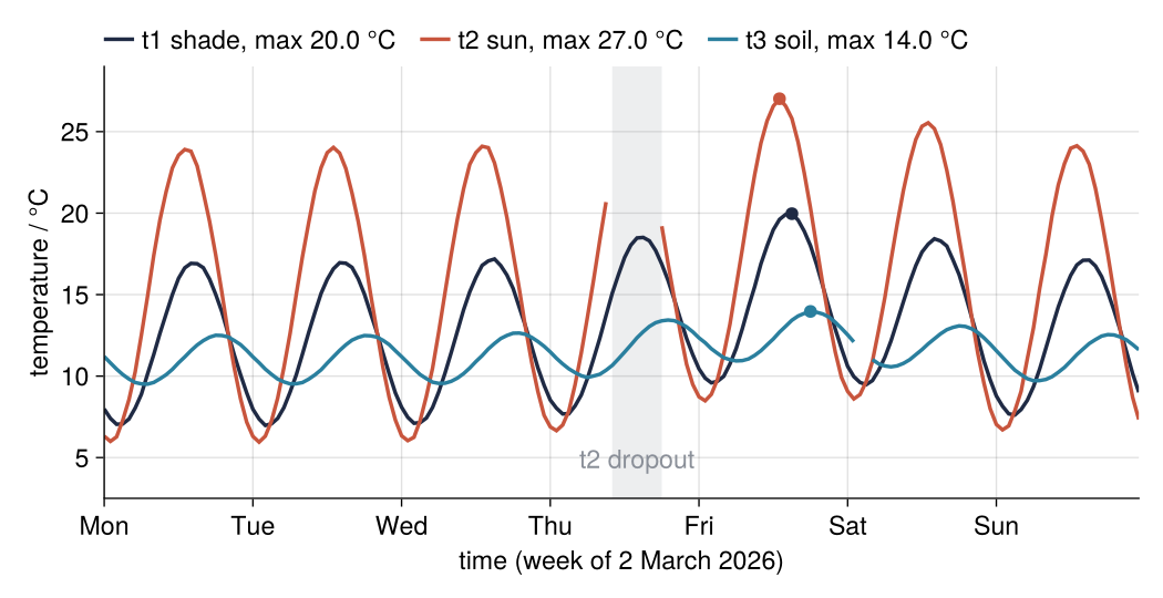
The last step draws this figure. Each line has 168 points, one mean per clock hour of the cleaned file, and a dot sits on each sensor's hottest hour, whose value the legend repeats. Where a sensor dropped out its line stops, and I kept those gaps visible deliberately. You need Julia arrays, functions, for loops, and broadcasting with the dot; nothing about DataFrames is assumed.
Setup
Install the packages once with import Pkg; Pkg.add(["CSV", "DataFrames", "CairoMakie"]); Dates, Statistics, Random, and Printf ship with Julia. The block below plays the logger: it draws the week from Xoshiro(SEED), a seeded generator, so every run draws the same numbers, and writes logger.csv. Its unfamiliar lines, allowmissing!, .= missing, and names with a colon such as :t2, are explained in the steps that use them. Julia's generator draws other numbers than NumPy's, so the values differ from the pandas version of this tutorial while the week has the same shape.
using CSV, DataFrames, Dates, Statistics, Random, Printf, CairoMakie

const SEED = 20261006

const INK, ACCENT, SECOND, MUTED = "#1f2a44", "#c8553d", "#2a7f9e", "#8a8f98"
set_theme!(Theme(                          # the look of every figure below
    size = (770, 396), fontsize = 17,
    palette = (color = [INK, ACCENT, SECOND, MUTED],),
    Axis = (topspinevisible = false, rightspinevisible = false, xgridvisible = true, ygridvisible = true),
    Lines = (linewidth = 2.5,),
))

# ---- the logger: one week, one row per minute
rng = Xoshiro(SEED)
N = 10_080
times = DateTime(2026, 3, 2) .+ Minute.(0:N-1)
hour_of_day = hour.(times) .+ minute.(times) ./ 60
day = Dates.value.(times .- times[1]) ./ 86_400_000      # milliseconds per day
spell = 3 .* exp.(-((day .- 4.6) ./ 1.2) .^ 2)          # a warm spell peaking on Friday

sensor(level, amp, peak_hour, noise, spell) =
    level .+ amp .* cos.(2π .* (hour_of_day .- peak_hour) ./ 24) .+ spell .+ noise .* randn(rng, N)

logger = DataFrame(time = times, status = 0,
                   t1 = round.(sensor(12, 5, 15, 0.3, spell); digits = 2),          # air, shade
                   t2 = round.(sensor(15, 9, 13.5, 0.5, spell); digits = 2),        # air, sun
                   t3 = round.(sensor(11, 1.5, 19, 0.1, spell ./ 2); digits = 2))   # soil, 10 cm
glitch = randperm(rng, N)[1:12]
logger[glitch, :status] .= 2
logger[glitch, [:t1, :t2, :t3]] .= 85.0                  # what the logger writes on a glitch
allowmissing!(logger, [:t2, :t3])
logger[DateTime(2026, 3, 5, 10, 23) .<= times .<= DateTime(2026, 3, 5, 17, 40), :t2] .= missing
logger[DateTime(2026, 3, 7, 2, 10) .<= times .<= DateTime(2026, 3, 7, 3, 39), :t3] .= missing
CSV.write("logger.csv", logger; dateformat = "yyyy-mm-dd HH:MM:SS")

@printf("wrote %d rows to logger.csv\n", nrow(logger))
wrote 10080 rows to logger.csv
Step 1: Read the file with CSV.read into a DataFrame
Look at the raw file first, a header line and then one line per minute:
readlines("logger.csv")[1:3]
3-element Vector{String}:
 "time,status,t1,t2,t3"
 "2026-03-02 00:00:00,0,8.54,6.49,11.44"
 "2026-03-02 00:01:00,0,7.8,5.84,11.55"
CSV.read builds the table. The second argument says what to build, and the keyword types makes time a DateTime, the type Dates works with, where CSV.jl alone would pick its own timestamp type:
df = CSV.read("logger.csv", DataFrame; types = Dict(:time => DateTime))
size(df)
(10080, 5)
:time is a Symbol, a name written as a value, and DataFrames.jl names every column with one. :time => DateTime is a Pair, a left and a right side joined by =>, and a Dict is built from Pairs. They return in Step 5 with a function in the middle. describe gives one row per column with the statistics named after df, and first(df, 3) shows the top rows:
describe(df, :eltype, :nmissing, :max)
| Row | variable | eltype | nmissing | max |
|---|---|---|---|---|
| Symbol | Type | Int64 | Any | |
| 1 | time | DateTime | 0 | 2026-03-08T23:59:00 |
| 2 | status | Int64 | 0 | 2 |
| 3 | t1 | Float64 | 0 | 85.0 |
| 4 | t2 | Union{Missing, Float64} | 438 | 85.0 |
| 5 | t3 | Union{Missing, Float64} | 90 | 85.0 |
first(df, 3)
| Row | time | status | t1 | t2 | t3 |
|---|---|---|---|---|---|
| DateTime | Int64 | Float64 | Float64? | Float64? | |
| 1 | 2026-03-02T00:00:00 | 0 | 8.54 | 6.49 | 11.44 |
| 2 | 2026-03-02T00:01:00 | 0 | 7.8 | 5.84 | 11.55 |
| 3 | 2026-03-02T00:02:00 | 0 | 8.24 | 6.58 | 11.34 |
An empty field becomes the value missing. The element type of t2 and t3 is therefore Union{Missing, Float64}, a number or missing, which first abbreviates to Float64?; t2 has 438 of them and t3 has 90. t1 is plain Float64 because its column in the file has no empty field, which matters in Step 3. All three maxima are 85.0.
Step 2: Select rows and columns by number, name, and condition
A DataFrame in Julia has no row index: rows have numbers, not labels. Indexing takes rows first and columns second. Rows are a number, a range, or a vector of Bool; columns are a name, a vector of names, or : for all of them:
df[1:3, [:time, :t2]]
| Row | time | t2 |
|---|---|---|
| DateTime | Float64? | |
| 1 | 2026-03-02T00:00:00 | 6.49 |
| 2 | 2026-03-02T00:01:00 | 5.84 |
| 3 | 2026-03-02T00:02:00 | 6.58 |
println(df[1, :t2])        # one row, one column: a single value
col = df[:, :t1]           # a copy of the column
col[1] = -99.0
println(df[1, :t1])        # df is unchanged
6.49
8.54
Whether indexing copies follows three rules. First, reading with brackets copies whenever the row position holds :, a range, or a vector: df[:, :t1] is a new vector, which is why setting col[1] left df alone. Second, df.t1, df[!, :t1], and a single row df[1, :] point into df itself; a ! for the rows means all of them, uncopied. Third, brackets directly left of = or .= write into df.
A condition selects rows when it is a Bool vector with one entry per row, which broadcasting builds:
hot = df[df.t1 .> 18, :]
@printf("%d minutes above 18 °C, %d of them flagged\n", nrow(hot), count(hot.status .!= 0))
825 minutes above 18 °C, 12 of them flagged
In the shade, 825 minutes exceed 18 °C and 12 of those carry a flag: all twelve glitches, because a glitch reads 85.0 °C. The same mechanism on the time column cuts out a window, six minutes on Thursday morning:
df[DateTime(2026, 3, 5, 10, 20) .<= df.time .<= DateTime(2026, 3, 5, 10, 25), :]
| Row | time | status | t1 | t2 | t3 |
|---|---|---|---|---|---|
| DateTime | Int64 | Float64 | Float64? | Float64? | |
| 1 | 2026-03-05T10:20:00 | 0 | 14.57 | 21.95 | 10.51 |
| 2 | 2026-03-05T10:21:00 | 0 | 15.05 | 22.99 | 10.61 |
| 3 | 2026-03-05T10:22:00 | 0 | 15.06 | 23.52 | 10.67 |
| 4 | 2026-03-05T10:23:00 | 0 | 14.42 | missing | 10.82 |
| 5 | 2026-03-05T10:24:00 | 0 | 15.38 | missing | 10.62 |
| 6 | 2026-03-05T10:25:00 | 0 | 15.03 | missing | 10.46 |
From 10:23 on, t2 reads missing: the dropout has begun.
Step 3: Mask the bad readings, and make room for missing
The shade sensor's maximum shows the problem:
maximum(df.t1)
85.0
No March shade reaches 85.0 °C; that reading comes from the logger. The status column marks the rows to distrust, and comparing it with the good code gives a mask, a Bool vector with one entry per row:
bad = df.status .!= 0          # anything but 0, the good code
println(count(bad), " flagged rows")
first(df[bad, :], 3)
12 flagged rows
| Row | time | status | t1 | t2 | t3 |
|---|---|---|---|---|---|
| DateTime | Int64 | Float64 | Float64? | Float64? | |
| 1 | 2026-03-03T02:54:00 | 2 | 85.0 | 85.0 | 85.0 |
| 2 | 2026-03-03T10:33:00 | 2 | 85.0 | 85.0 | 85.0 |
| 3 | 2026-03-03T17:22:00 | 2 | 85.0 | 85.0 | 85.0 |
Writing missing into the bad rows of the sensor columns is one line, and it fails. try catches the error so that the notebook runs on:
sensors = [:t1, :t2, :t3]
try
    df[bad, sensors] .= missing
catch err
    println(split(sprint(showerror, err), "\n")[1])    # first line of the error message
end
MethodError: Cannot `convert` an object of type Missing to an object of type Float64
A Float64 column holds numbers only, and t1 is one. allowmissing! widens the element type to Union{Missing, Float64} first. A ! has three meanings here: at the end of a function name, by Julia's convention, a function that changes its argument; in front of a value, as in !ismissing(x) and !=, "not"; in the row position, df[!, :t1], all rows without a copy.
allowmissing!(df, sensors)
df[bad, sensors] .= missing
count(ismissing.(df.t1))
12
The write reaches df because the brackets stand directly left of .=. I mark the readings as missing instead of deleting the rows: every minute keeps its row, and missing is already how the file records a lost reading. Split into two indexing steps, the same write changes nothing; the first pitfall shows it.
Step 4: Count what is missing, and decide what to skip
Ask for the mean of the shade sensor:
mean(df.t1)
missing
The answer is missing. A missing passes through arithmetic and through mean, maximum, and sum, so that a missing value is never ignored without your say. skipmissing is how you say it:
mean(skipmissing(df.t1))
12.906925903853807
count(ismissing, col) hands count the function itself, without parentheses, and count applies it to every element: the number of Step 3 without building a Bool vector first. mean(ismissing, col) gives the fraction:
missing_pct = Float64[]
for s in sensors
    col = df[:, s]                          # a copy, harmless for reading
    push!(missing_pct, 100 * mean(ismissing, col))
    @printf("%s: %4d minutes missing, %5.2f %%, max %.2f °C\n",
            s, count(ismissing, col), missing_pct[end], maximum(skipmissing(col)))
end
t1:   12 minutes missing,  0.12 %, max 20.79 °C
t2:  450 minutes missing,  4.46 %, max 28.21 °C
t3:  101 minutes missing,  1.00 %, max 14.19 °C
Every sensor lost its 12 glitch minutes. On top of those, t2 lost 438 minutes to its dropout and t3 lost 90, one of which was already a glitch, hence 101 and not 102. The maxima are weather now. What to skip is your decision, and skipping across the whole table is the wrong one:
kept = dropmissing(df)
@printf("dropmissing(df):      %d of %d rows kept\n", nrow(kept), nrow(df))
@printf("dropmissing(df, :t1): %d rows kept\n", nrow(dropmissing(df, :t1)))
@printf("t1 mean, every valid minute: %.2f °C\n", mean(skipmissing(df.t1)))
@printf("t1 mean after dropmissing:   %.2f °C\n", mean(kept.t1))
dropmissing(df):      9541 of 10080 rows kept
dropmissing(df, :t1): 10068 rows kept
t1 mean, every valid minute: 12.91 °C
t1 mean after dropmissing:   12.72 °C
dropmissing(df) throws out every row in which any column holds missing. The shade sensor thereby pays 527 good minutes for the dropouts of the other two, mostly from a warm Thursday afternoon, and its mean falls from 12.91 to 12.72 °C. dropmissing(df, :t1) checks one column only. Skip per computation, not per table. skipmissing never reports how many values remained; the next step counts them.
Step 5: Average by clock hour with groupby, combine, and a coverage rule
An hourly mean is a grouping by a computed column: floor rounds each timestamp down to the start of its clock hour, 10:37 to 10:00. Assigning to a new name adds a column:
df.hour = floor.(df.time, Hour)
g = groupby(df, :hour)
println(length(g), " groups")
168 groups
groupby sorts the rows into 168 groups and computes nothing. combine does the work, with the Pair of Step 1 and a function in the middle, source => function => target. The function receives the column of one group, and its result becomes that group's value in the target column. The dot in .=> broadcasts over the three names and makes three Pairs. First the valid minutes per hour:
nvalid(x) = length(x) - count(ismissing, x)
counts = combine(g, sensors .=> nvalid .=> sensors)
counts[DateTime(2026, 3, 5, 9) .<= counts.hour .<= DateTime(2026, 3, 5, 18), :]
| Row | hour | t1 | t2 | t3 |
|---|---|---|---|---|
| DateTime | Int64 | Int64 | Int64 | |
| 1 | 2026-03-05T09:00:00 | 60 | 60 | 60 |
| 2 | 2026-03-05T10:00:00 | 60 | 23 | 60 |
| 3 | 2026-03-05T11:00:00 | 60 | 0 | 60 |
| 4 | 2026-03-05T12:00:00 | 60 | 0 | 60 |
| 5 | 2026-03-05T13:00:00 | 60 | 0 | 60 |
| 6 | 2026-03-05T14:00:00 | 60 | 0 | 60 |
| 7 | 2026-03-05T15:00:00 | 60 | 0 | 60 |
| 8 | 2026-03-05T16:00:00 | 60 | 0 | 60 |
| 9 | 2026-03-05T17:00:00 | 60 | 19 | 60 |
| 10 | 2026-03-05T18:00:00 | 60 | 60 | 60 |
Six hours of t2 are empty. The hours at 10:00 and 17:00 kept 23 and 19, and a mean from those would pass for an hourly value while covering only the first or last part of the hour. Require coverage, here 45 of 60 minutes; choose the threshold from how fast the quantity changes within one bin, and state it with the result. cond ? a : b gives a if the condition holds, else b.
The loop that follows finds each sensor's hottest hour. findmax returns the largest value and its position, and skipmissing passes over the missing entries but keeps their numbering, so i is a row of hourly; the format "e HH:MM" prints its hour as weekday (e), hour, and minute:
covered_mean(x) = nvalid(x) >= 45 ? mean(skipmissing(x)) : missing
hourly = combine(g, sensors .=> covered_mean .=> sensors)
println(size(hourly))

hottest_hour, peak, peak_row = String[], Float64[], Int[]
for s in sensors
    v, i = findmax(skipmissing(hourly[:, s]))
    push!(hottest_hour, Dates.format(hourly.hour[i], "e HH:MM"))
    push!(peak, v)
    push!(peak_row, i)
    @printf("%s: %d hours without a mean, hottest hour %s, %.2f °C\n",
            s, count(ismissing, hourly[:, s]), hottest_hour[end], v)
end
(168, 4)
t1: 0 hours without a mean, hottest hour Fri 15:00, 19.96 °C
t2: 8 hours without a mean, hottest hour Fri 13:00, 27.02 °C
t3: 2 hours without a mean, hottest hour Fri 18:00, 13.97 °C
Friday holds all three maxima, the soil's three hours after the shade's. t2 lacks eight means, six empty hours and two thin ones; t3 lacks Saturday 02:00 and 03:00, with 10 and 20 minutes.
Step 6: Group by hour of day, then tabulate, plot, and save
Any column can be grouped on. hour.(df.time) is the hour of day of each row, 0 to 23, and grouping on it averages all minutes that share a clock hour across the seven days. The line for warmest is a comprehension, a for loop inside brackets that collects its results in a vector; argmax gives only the position:
df.hourofday = hour.(df.time)
skipmean(x) = mean(skipmissing(x))
cycle = combine(groupby(df, :hourofday), sensors .=> skipmean .=> sensors)
warmest = [cycle.hourofday[argmax(cycle[:, s])] for s in sensors]
println(size(cycle), ", warmest hour of day: ", warmest)
cycle[13:20, :]
(24, 4), warmest hour of day: [15, 13, 18]
| Row | hourofday | t1 | t2 | t3 |
|---|---|---|---|---|
| Int64 | Float64 | Float64 | Float64 | |
| 1 | 12 | 16.8644 | 24.4762 | 11.259 |
| 2 | 13 | 17.514 | 24.7887 | 11.6469 |
| 3 | 14 | 17.8375 | 24.5073 | 12.0239 |
| 4 | 15 | 17.8411 | 23.6211 | 12.3673 |
| 5 | 16 | 17.5311 | 22.0902 | 12.6444 |
| 6 | 17 | 16.8494 | 20.2594 | 12.8308 |
| 7 | 18 | 15.9501 | 18.2524 | 12.9443 |
| 8 | 19 | 14.8198 | 15.9503 | 12.9323 |
On a typical day the sun sensor is warmest at 13:00 and the shade air at 15:00, while the soil waits until 18:00, three to five hours behind the air. Grouping on a site or treatment column, groupby(df, :treatment), works the same way. The summary puts the vectors of Steps 4 to 6 side by side, one keyword per column:
report = DataFrame(sensor = sensors, missing_pct = round.(missing_pct; digits = 2),
                   hottest_hour = hottest_hour, max_C = round.(peak; digits = 2),
                   warmest_hour_of_day = warmest)
| Row | sensor | missing_pct | hottest_hour | max_C | warmest_hour_of_day |
|---|---|---|---|---|---|
| Symbol | Float64 | String | Float64 | Int64 | |
| 1 | t1 | 0.12 | Fri 15:00 | 19.96 | 15 |
| 2 | t2 | 4.46 | Fri 13:00 | 27.02 | 13 |
| 3 | t3 | 1.0 | Fri 18:00 | 13.97 | 18 |
The plot is ordinary Makie on the columns of hourly, and the Makie documentation explains each call. Only coalesce.(hourly[:, s], NaN) belongs to this tutorial: it turns missing into NaN, which Makie draws as a gap:
hours = 0:nrow(hourly)-1                  # one row per hour, in order from Monday 00:00
labels = Dict(:t1 => "t1 shade", :t2 => "t2 sun", :t3 => "t3 soil")
fig = Figure()
ax = Axis(fig[1, 1]; xlabel = "time (week of 2 March 2026)", ylabel = "temperature / °C",
          xticks = (0:24:144, ["Mon", "Tue", "Wed", "Thu", "Fri", "Sat", "Sun"]))
vspan!(ax, 3 * 24 + 10, 3 * 24 + 18; color = (MUTED, 0.15))
text!(ax, 3 * 24 + 14, 4; text = "t2 dropout", color = MUTED, align = (:center, :bottom))
for (k, (s, color)) in enumerate(zip(sensors, [INK, ACCENT, SECOND]))
    lines!(ax, hours, coalesce.(hourly[:, s], NaN); color,
           label = @sprintf("%s, max %.1f °C", labels[s], peak[k]))
    scatter!(ax, [hours[peak_row[k]]], [peak[k]]; color, markersize = 12)
end
xlims!(ax, 0, 167)
ylims!(ax, 2.5, 29)
Legend(fig[0, 1], ax; orientation = :horizontal, framevisible = false, halign = :left, padding = 0)
rowgap!(fig.layout, 8)                    # pixels between legend and axes
fig
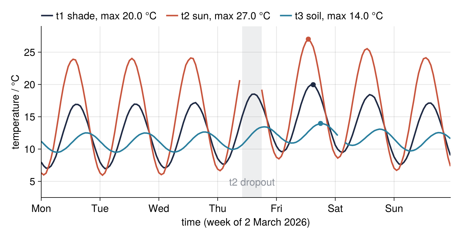
On Friday the warm spell adds about 3 °C to both air sensors and about 1.5 °C to the soil. CSV.write saves the cleaned table without the helper columns, and each missing becomes an empty field again, as the first glitch row shows:
CSV.write("logger_clean.csv", df[:, [:time, :status, :t1, :t2, :t3]])
readlines("logger_clean.csv")[[1, 2, 1 + findfirst(bad)]]
3-element Vector{String}:
 "time,status,t1,t2,t3"
 "2026-03-02T00:00:00,0,8.54,6.49,11.44"
 "2026-03-03T02:54:00,2,,,"
Pitfalls
Assigning into a selection changes a copy. Mask the glitches in two indexing steps, rows first and then the column, and Julia runs it without a word. Here it is on the raw file read in again, where t2 already allows missing:
raw = CSV.read("logger.csv", DataFrame; types = Dict(:time => DateTime))
raw[raw.status .!= 0, :].t2 .= missing
maximum(skipmissing(raw.t2))
85.0
The maximum of t2 is still 85.0 °C, so the glitches survived. By the rule of Step 2, the brackets are followed by .t2, so they are read from, and with a vector of rows they build a new DataFrame; the .= writes into that one, which is then thrown away. The fix is one indexing call, raw[bad, :t2] .= missing. When a selection must write through, take view(raw, bad, :), a selection that points into raw instead of copying it.
A daily mean that hides a gap. floor.(df.time, Day) gives daily groups. Here is the daily mean of t2 with its count of valid minutes, next to the truth, the generated curve before noise, rebuilt from the setup's hour_of_day and spell:
df.day = floor.(df.time, Day)
daily = combine(groupby(df, :day), :t2 => skipmean => :mean, :t2 => nvalid => :minutes)
truth = 15 .+ 9 .* cos.(2π .* (hour_of_day .- 13.5) ./ 24) .+ spell
daily.truth = [mean(truth[floor.(times, Day) .== d]) for d in daily.day]
daily
| Row | day | mean | minutes | truth |
|---|---|---|---|---|
| DateTime | Float64 | Int64 | Float64 | |
| 1 | 2026-03-02T00:00:00 | 14.9832 | 1440 | 15.0001 |
| 2 | 2026-03-03T00:00:00 | 15.0025 | 1437 | 15.0069 |
| 3 | 2026-03-04T00:00:00 | 15.1663 | 1438 | 15.1822 |
| 4 | 2026-03-05T00:00:00 | 12.9689 | 1002 | 16.3398 |
| 5 | 2026-03-06T00:00:00 | 17.8253 | 1437 | 17.8175 |
| 6 | 2026-03-07T00:00:00 | 16.7185 | 1439 | 16.7184 |
| 7 | 2026-03-08T00:00:00 | 15.2922 | 1437 | 15.301 |
On Thursday the mean is 12.97 °C, computed from 1,002 minutes, while the truth is 16.34 °C. The lost minutes are the warm part of that day, and the mean alone gives no sign of it. Step 5's coverage rule fixes it, with a threshold sized for a day, for instance nvalid(x) >= 1200. A period with no rows at all does not appear as a group, so for a logger that skips rows instead of writing empty fields, count the rows per period too.
A time column that is text. A logger that writes 02.03.2026 00:00 does not use the ISO form, and CSV.jl leaves the column as text. Everything looks fine until floor.(df.time, Hour) raises MethodError: no method matching floor(::DataStrings.DataString, ::Type{Hour}). Pass dateformat = "dd.mm.yyyy HH:MM" together with types = Dict(:time => DateTime), and look at describe(df) before anything else. The same European export often separates fields with ; and writes 12,5; delim = ';' and decimal = ',' read it.
Variations
- Several files, one table. When the logger starts a new file every day,
CSV.read(sort(paths), DataFrame; types = Dict(:time => DateTime))takes a vector of paths and stacks the files into one table. - Many sensors or sites, in long form.
long = stack(df, sensors, [:time, :hour])gives one row per reading, with the sensor name invariableand the reading invalue;groupby(long, [:variable, :hour])then groups by sensor and by hour together. - Join a table of sensor metadata. With a table
metathat has one row per sensor and avariablecolumn,leftjoin(long, meta, on = :variable)adds depth, exposure, or calibration offset to every reading. - Rolling means. DataFrames.jl has no rolling window; RollingFunctions.jl has one, and
[skipmean(col[i-29:i]) for i in 30:length(col)]is a 30-minute mean by hand.
Cheat sheet
df = CSV.read(path, DataFrame; types = Dict(:time => DateTime))  # delim, decimal, dateformat
describe(df, :eltype, :nmissing)                    # check types and gaps first
df[rows, cols];  df[df.t1 .> 18, :]                 # numbers, names, Bool vectors
allowmissing!(df, cols);  df[mask, cols] .= missing # one indexing call, never df[mask, :].t1 .= ...
mean(skipmissing(x));  count(ismissing, x)          # skip on purpose; count the gaps
dropmissing(df, :t1)                                # drop per column, not per table
df.hour = floor.(df.time, Hour)                     # the clock hour of every row
combine(groupby(df, :hour), cols .=> f .=> cols)    # f gets one group's column
v, i = findmax(skipmissing(x));  CSV.write(path, df)  # value and position; write out
Further reading
- The DataFrames.jl manual: Getting Started, Working with DataFrames, and The Split-Apply-Combine Strategy; the Julia manual on Missing Values.
- The CSV.jl documentation on
CSV.readand itstypes,dateformat,delim, anddecimalkeywords, and the Makie documentation for the figure. - Bogumił Kamiński, Julia for Data Analysis (Manning, 2023).
- Related tutorials on this site: pandas from the ground up: a week of temperature logs, the same week in Python; Fit a curve with error bars and draw a confidence band in Julia, for what to do with clean numbers; The Fourier transform in Julia: asking a signal how much of each frequency it contains, another sampled time series with a seeded
Xoshiro. - Download the notebook. It was executed with the library versions in the header.