pandas from the ground up: a week of temperature logs
Afterwards you can read a table into a pandas DataFrame, select by label and condition, handle missing values deliberately, and average by hour or group.
- Topic
- Data wrangling
- Field
- Cross-disciplinary
- Prerequisites
- none beyond Python basics
- Libraries
matplotlib 3.11.2numpy 2.5.3pandas 3.0.6
py-pandas.ipynb, executed with the versions above
The problem: what happened in a week of temperature logs
A data logger at a field station recorded three temperature sensors once a minute for one week, Monday 2 March 2026 to Sunday 23:59. That is 10,080 rows of a timestamp, a status code, and three readings: t1 air in the shade, t2 air in the sun, t3 soil at 10 cm. You want to know what fraction of each sensor is missing, what the hourly means look like, in which hour of the week each sensor was hottest, and at which hour of an average day. With pandas each answer is a few lines once the file is a DataFrame, a table whose columns have names and whose rows have labels.
The file contains two kinds of bad data. Twelve rows carry status 2 instead of the good 0, a logger glitch, and read 85.0 °C on all three sensors. Leave them in and every sensor's maximum is 85.0 °C, in the soil, in March. The other kind is a gap where a sensor dropped out and the field is empty, seven hours of t2 on Thursday and an hour and a half of t3 early on Saturday. Every measuring field produces files like this, from a plate reader to a weather mast.
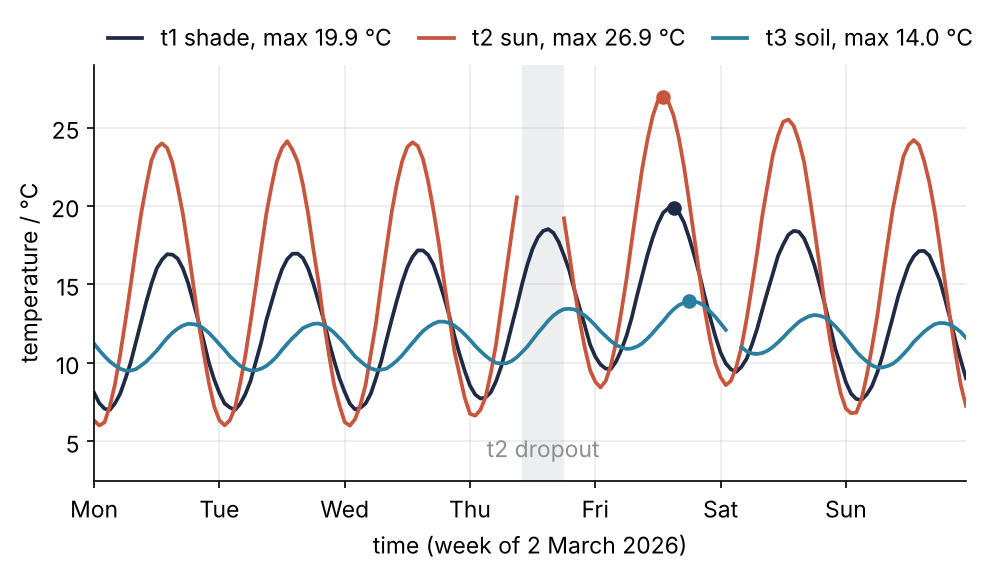
This is where we end up: 168 hourly means per sensor, the hottest hour of each marked with a dot and its value in the legend. The breaks in t2 on Thursday and in t3 early on Saturday are the dropouts, left as breaks on purpose. Each point averages one clock hour of the cleaned file.
Setup
The block below plays the logger: it builds the week with a seeded generator from default_rng and writes logger.csv. From the next step on we work from the file alone, until the second pitfall needs the noise-free truth from three of the setup's variables.
import numpy as np
import pandas as pd
import matplotlib.pyplot as plt
import matplotlib.dates as mdates

SEED = 20261006

plt.rcParams.update({
    "figure.figsize": (7.5, 3.6), "figure.dpi": 110,
    "axes.spines.top": False, "axes.spines.right": False,
    "axes.grid": True, "grid.alpha": 0.25,
    "font.size": 11, "lines.linewidth": 1.8,
})
INK, ACCENT, SECOND, MUTED = "#1f2a44", "#c8553d", "#2a7f9e", "#8a8f98"

# ---- the logger: one week, one row per minute
rng = np.random.default_rng(SEED)
time = pd.date_range("2026-03-02", periods=10_080, freq="min")
hour_of_day = time.hour + time.minute / 60
day = (time - time[0]) / pd.Timedelta("1D")
spell = 3 * np.exp(-((day - 4.6) / 1.2) ** 2)          # a warm spell peaking on Friday

def sensor(mean, amp, peak_hour, noise, spell):
    cycle = amp * np.cos(2 * np.pi * (hour_of_day - peak_hour) / 24)
    return mean + cycle + spell + rng.normal(0, noise, time.size)

log = pd.DataFrame({"time": time, "status": 0,
                    "t1": sensor(12, 5, 15, 0.3, spell),          # air, shade
                    "t2": sensor(15, 9, 13.5, 0.5, spell),        # air, sun
                    "t3": sensor(11, 1.5, 19, 0.1, spell / 2)})   # soil, 10 cm
glitch = rng.choice(len(log), size=12, replace=False)
log.loc[glitch, "status"] = 2
log.loc[glitch, ["t1", "t2", "t3"]] = 85.0                        # what the logger writes on a glitch
log.loc[(time >= "2026-03-05 10:23") & (time <= "2026-03-05 17:40"), "t2"] = np.nan
log.loc[(time >= "2026-03-07 02:10") & (time <= "2026-03-07 03:39"), "t3"] = np.nan
log[["t1", "t2", "t3"]] = log[["t1", "t2", "t3"]].round(2)
log.to_csv("logger.csv", index=False)

print(f"pandas {pd.__version__}, wrote {len(log):,} rows to logger.csv")
pandas 3.0.6, wrote 10,080 rows to logger.csv
Step 1: Read the file with read_csv and parse_dates
Look at the raw file first. It is plain text, one line per minute, with a header line naming the columns:
with open("logger.csv") as f:
    print("".join(f.readline() for _ in range(3)))
time,status,t1,t2,t3
2026-03-02 00:00:00,0,8.3,6.51,11.29
2026-03-02 00:01:00,0,8.08,6.84,11.48
pd.read_csv turns it into a DataFrame. Without help it would read the first column as text, so parse_dates names the columns that hold times:
df = pd.read_csv("logger.csv", parse_dates=["time"])
print(df.shape)
print(df.dtypes)
(10080, 5)
time      datetime64[us]
status             int64
t1               float64
t2               float64
t3               float64
dtype: object
df.head()
| time | status | t1 | t2 | t3 | |
|---|---|---|---|---|---|
| 0 | 2026-03-02 00:00:00 | 0 | 8.30 | 6.51 | 11.29 |
| 1 | 2026-03-02 00:01:00 | 0 | 8.08 | 6.84 | 11.48 |
| 2 | 2026-03-02 00:02:00 | 0 | 8.66 | 6.25 | 11.45 |
| 3 | 2026-03-02 00:03:00 | 0 | 8.58 | 7.06 | 11.29 |
| 4 | 2026-03-02 00:04:00 | 0 | 8.16 | 6.34 | 11.41 |
Five columns and 10,080 rows. The time column is datetime64[us], timestamps at microsecond resolution, the readings are float64, and the empty fields of the dropouts came in as NaN, as the next step shows. A DataFrame is a set of named columns that share one row index, the row labels at the left. Here they are just the numbers 0 to 10,079. Each column on its own is a Series, a NumPy-like array that carries the same labels.
Step 2: Put time on the index and select with loc and iloc
Row numbers say nothing about the measurement. The time does, so make it the index:
df = df.set_index("time")
df.loc["2026-03-05 10:20":"2026-03-05 10:25"]
| status | t1 | t2 | t3 | |
|---|---|---|---|---|
| time | ||||
| 2026-03-05 10:20:00 | 0 | 14.29 | 21.84 | 10.67 |
| 2026-03-05 10:21:00 | 0 | 15.17 | 21.99 | 10.68 |
| 2026-03-05 10:22:00 | 0 | 15.30 | 22.54 | 10.65 |
| 2026-03-05 10:23:00 | 0 | 14.64 | NaN | 10.64 |
| 2026-03-05 10:24:00 | 0 | 15.57 | NaN | 10.57 |
| 2026-03-05 10:25:00 | 0 | 14.99 | NaN | 10.71 |
loc selects by label. pandas parses the two strings into timestamps and compares them with the index, and a label slice includes both ends, so you get six minutes. The t2 dropout starts at 10:23. Rows come first and columns second, both for loc and for its positional twin iloc:
print(df.loc["2026-03-05 10:20", "t2"])      # one row label, one column label
print(df.iloc[0, 1])                         # first row, second column
df.iloc[:3]
21.84
8.3
| status | t1 | t2 | t3 | |
|---|---|---|---|---|
| time | ||||
| 2026-03-02 00:00:00 | 0 | 8.30 | 6.51 | 11.29 |
| 2026-03-02 00:01:00 | 0 | 8.08 | 6.84 | 11.48 |
| 2026-03-02 00:02:00 | 0 | 8.66 | 6.25 | 11.45 |
Plain brackets follow a two-part rule. A column name or a list of names selects columns: df["t1"] is a Series, df[["t1", "t2"]] a DataFrame. A boolean Series with one value per row selects rows:
print(type(df["t1"]).__name__, type(df[["t1", "t2"]]).__name__)
above = df[df["t1"] > 18]
print(above.shape, "of which status 2:", (above["status"] == 2).sum())
Series DataFrame
(814, 4) of which status 2: 12
814 minutes above 18 °C in the shade, 12 of them glitches. That is every glitch in the file, since each one reads 85.0 °C. The next step removes them.
Step 3: Mask the bad readings with a boolean condition
The maxima show the problem at once:
sensors = ["t1", "t2", "t3"]
df[sensors].max()
t1    85.0
t2    85.0
t3    85.0
dtype: float64
85.0 °C in the soil in March is a glitch, not weather. The status column says which rows to distrust, and a comparison turns it into a mask, the row selection of Step 2:
bad = df["status"] != 0          # anything but 0, the good code
print(bad.sum(), "flagged rows")
df[bad].head(3)
12 flagged rows
| status | t1 | t2 | t3 | |
|---|---|---|---|---|
| time | ||||
| 2026-03-02 09:00:00 | 2 | 85.0 | 85.0 | 85.0 |
| 2026-03-03 02:35:00 | 2 | 85.0 | 85.0 | 85.0 |
| 2026-03-04 07:22:00 | 2 | 85.0 | 85.0 | 85.0 |
One loc call with the mask for the rows and the list for the columns selects the cells and assigns to them:
df.loc[bad, sensors] = np.nan
df[sensors].max()
t1    20.65
t2    27.90
t3    14.21
dtype: float64
Now the maxima are 20.65, 27.90, and 14.21 °C, which is weather. I set the readings to NaN instead of dropping the rows, for two reasons: the timeline stays whole, one row per minute, and NaN is already what the file uses for a missing reading, so one convention covers both kinds of bad data. The assignment has to be one loc call. Selecting the rows first and then assigning to a column of the result, df[bad]["t1"] = np.nan, does nothing, as the first pitfall shows.
Step 4: Count what is missing with isna, and decide what to do with it
isna() returns a table of booleans, True where a value is missing. Summed, it counts; averaged, it gives the fraction:
n_missing = df[sensors].isna().sum()
pct_missing = df[sensors].isna().mean() * 100
for s in sensors:
    print(f"{s}: {n_missing[s]:4d} minutes missing, {pct_missing[s]:5.2f} %")
t1:   12 minutes missing,  0.12 %
t2:  450 minutes missing,  4.46 %
t3:  102 minutes missing,  1.01 %
The 12 glitches in every sensor, plus 438 minutes of dropout in t2 and 90 in t3. What to do with them is a decision, and the obvious one is wrong:
kept = df.dropna()
print(f"dropna():              {len(kept):,} of {len(df):,} rows kept")
print(f"dropna(subset=['t1']): {len(df.dropna(subset=['t1'])):,} rows kept")
print(f"t1 mean, every valid minute: {df['t1'].mean():.2f} °C")
print(f"t1 mean after dropna():      {kept['t1'].mean():.2f} °C")
dropna():              9,540 of 10,080 rows kept
dropna(subset=['t1']): 10,068 rows kept
t1 mean, every valid minute: 12.91 °C
t1 mean after dropna():      12.73 °C
dropna() drops a row when any column is missing, so the shade sensor loses 528 good minutes because the other two failed, and its mean moves from 12.91 to 12.73 °C. Most of what it lost is a warm Thursday afternoon, so the mean drops. If you drop at all, drop per sensor with subset=. Most of the time you do not need to: mean() skips NaN on its own. What it does not tell you is how many values it used, and that is the subject of the next step.
Step 5: Resample to hourly means with a coverage rule
Resampling in pandas means something narrower than in statistics: cut the time index into bins of fixed length, here one clock hour labeled by its start, so 10:00 stands for 10:00 to 10:59, and summarize each bin. It is not drawing new samples. The call has two stages, and the first computes nothing:
r = df[sensors].resample("h")
print(r)
DatetimeIndexResampler [freq=<Hour>, closed=left, label=left, convention=start, origin=start_day]
The resampler only knows the bins. r.count() and r.mean() do the work, one row per hour, 168 rows. The counts for Thursday morning to evening show the dropout:
counts = r.count()
print(counts.shape)
counts.loc["2026-03-05 09:00":"2026-03-05 18:00"]
(168, 3)
| t1 | t2 | t3 | |
|---|---|---|---|
| time | |||
| 2026-03-05 09:00:00 | 60 | 60 | 60 |
| 2026-03-05 10:00:00 | 60 | 23 | 60 |
| 2026-03-05 11:00:00 | 60 | 0 | 60 |
| 2026-03-05 12:00:00 | 60 | 0 | 60 |
| 2026-03-05 13:00:00 | 60 | 0 | 60 |
| 2026-03-05 14:00:00 | 60 | 0 | 60 |
| 2026-03-05 15:00:00 | 60 | 0 | 60 |
| 2026-03-05 16:00:00 | 60 | 0 | 60 |
| 2026-03-05 17:00:00 | 60 | 19 | 60 |
| 2026-03-05 18:00:00 | 60 | 60 | 60 |
Six hours of t2 have no minute at all, and their mean is NaN. The hour at 10:00 has 23 minutes and the one at 17:00 has 19, and their means are worse than NaN: they look valid and describe only the start or the end of the hour. So demand coverage, at least 45 of 60 minutes per hour. DataFrame.where(cond) keeps a value where the condition holds and puts NaN elsewhere, and the two tables line up by their row and column labels, not by position:
hourly = r.mean().where(counts >= 45)
peak_time, peak = hourly.idxmax(), hourly.max()
for s in sensors:
    print(f"{s}: {hourly[s].isna().sum()} hours without a mean, "
          f"hottest hour {peak_time[s]:%a %H:%M}, {peak[s]:.2f} °C")
t1: 0 hours without a mean, hottest hour Fri 15:00, 19.91 °C
t2: 8 hours without a mean, hottest hour Fri 13:00, 26.93 °C
t3: 2 hours without a mean, hottest hour Fri 18:00, 13.95 °C
idxmax is np.argmax that returns the label instead of the position, here a timestamp, which %a %H:%M in the f-string prints as weekday, hour, and minute. All three sensors peak on Friday, in the warm spell, the soil three hours after the shade. The two t3 hours without a mean are Saturday 02:00 and 03:00, which kept 10 and 20 minutes. resample("D") gives daily means the same way.
Step 6: Group by hour of day, then tabulate, plot, and save
Resampling bins the time axis. Grouping bins by the values of any column. df.index.hour is the hour of each timestamp, an integer from 0 to 23 (.day_name() works the same), and as a column it can be grouped on:
df["hour"] = df.index.hour
cycle = df.groupby("hour")[sensors].mean()
print(cycle.shape)
print(cycle.loc[12:19].round(2))
print("warmest hour of day:", cycle.idxmax().to_dict())
(24, 3)
         t1     t2     t3
hour
12    16.86  24.52  11.26
13    17.50  24.81  11.65
14    17.84  24.46  12.03
15    17.85  23.56  12.37
16    17.55  22.13  12.64
17    16.88  20.29  12.83
18    15.96  18.23  12.94
19    14.83  15.94  12.93
warmest hour of day: {'t1': 15, 't2': 13, 't3': 18}
All minutes that share an hour of day are averaged, across the seven days, 24 rows. On an average day the sun sensor peaks at 13:00, the shade at 15:00, the soil at 18:00: the soil lags the air by three to five hours. A table with a site or treatment column groups the same way, df.groupby("treatment"). Now the summary. pd.DataFrame accepts a dict of Series: each key becomes a column name, and the Series are lined up by their labels, the sensor names t1 to t3, which become the rows:
summary = pd.DataFrame({
    "missing %": pct_missing.round(2),
    "hottest hour": peak_time,
    "max / °C": peak.round(2),
    "warmest hour of day": cycle.idxmax(),
})
summary
| missing % | hottest hour | max / °C | warmest hour of day | |
|---|---|---|---|---|
| t1 | 0.12 | 2026-03-06 15:00:00 | 19.91 | 15 |
| t2 | 4.46 | 2026-03-06 13:00:00 | 26.93 | 13 |
| t3 | 1.01 | 2026-03-06 18:00:00 | 13.95 | 18 |
The figure uses plain Matplotlib calls on the index and the columns, so it takes the styling of the setup. The date locators and the legend placement are explained in Matplotlib from the ground up:
fig, ax = plt.subplots()
ax.axvspan(pd.Timestamp("2026-03-05 10:00"), pd.Timestamp("2026-03-05 18:00"),
           color=MUTED, alpha=0.15, lw=0)
ax.text(pd.Timestamp("2026-03-05 14:00"), 4, "t2 dropout", color=MUTED, ha="center")
labels = {"t1": "t1 shade", "t2": "t2 sun", "t3": "t3 soil"}
for s, color in zip(sensors, [INK, ACCENT, SECOND]):
    ax.plot(hourly.index, hourly[s], color=color,
            label=f"{labels[s]}, max {peak[s]:.1f} °C")
    ax.plot(peak_time[s], peak[s], "o", color=color, ms=6)
ax.xaxis.set_major_locator(mdates.DayLocator())
ax.xaxis.set_major_formatter(mdates.DateFormatter("%a"))
ax.set(xlabel="time (week of 2 March 2026)", ylabel="temperature / °C",
       xlim=(hourly.index[0], hourly.index[-1]), ylim=(2.5, 29))
ax.legend(frameon=False, loc="lower left", bbox_to_anchor=(0, 1), ncols=3,
          handlelength=1.5, columnspacing=1.2, borderaxespad=0.2)
plt.show()
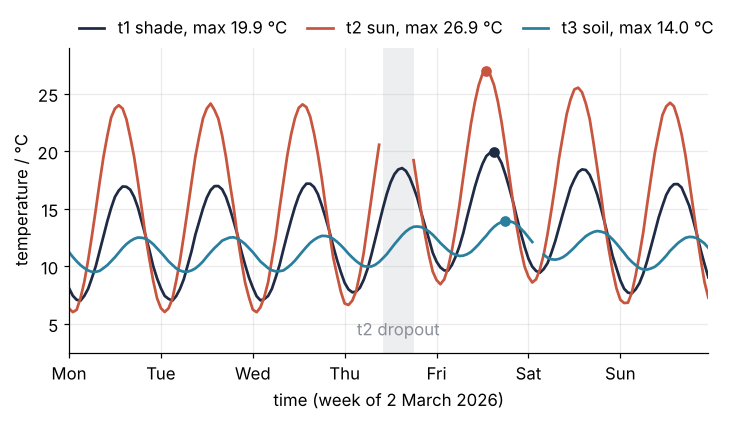
The warm spell lifts Friday by about 3 °C in the air and half that in the soil. Last, write the cleaned data back out, without the helper column; the index becomes the time column again:
df[["status"] + sensors].to_csv("logger_clean.csv")
with open("logger_clean.csv") as f:
    print("".join(f.readline() for _ in range(2)))
time,status,t1,t2,t3
2026-03-02 00:00:00,0,8.3,6.51,11.29
Pitfalls
Chained assignment does nothing. Mask the glitches in two steps, df[bad]["t1"] = np.nan, and Python runs it, pandas prints a warning, and the glitches are still there. Below, on a fresh read of the unmasked file (index_col="time" does the set_index of Step 2 in the same call):
raw = pd.read_csv("logger.csv", parse_dates=["time"], index_col="time")
raw[raw["status"] != 0]["t1"] = np.nan
print("t1 max:", raw["t1"].max())
t1 max: 85.0
ChainedAssignmentError: A value is being set on a copy of a DataFrame or Series through chained assignment.
Such chained assignment never works to update the original DataFrame or Series, because the intermediate object on which we are setting values always behaves as a copy (due to Copy-on-Write).

Try using '.loc[row_indexer, col_indexer] = value' instead, to perform the assignment in a single step.

See the documentation for a more detailed explanation: https://pandas.pydata.org/pandas-docs/stable/user_guide/copy_on_write.html#chained-assignment
raw[...] with a mask builds a new DataFrame, the assignment changes that new one, and raw never sees it. The fix is the one loc call of Step 3, df.loc[bad, "t1"] = np.nan. Answers written for pandas before 3.0 discuss this under SettingWithCopyWarning, which pandas 3 removed. In pandas 3 chained assignment never works, and the ChainedAssignmentError printed above says so. Despite its name it is a warning, not an exception: the cell runs to the end with the glitches in place.
A daily mean that hides a gap. The daily mean of t2, with its count beside it (agg computes several summaries at once), and the noise-free truth, rebuilt from time, hour_of_day, and spell of the setup cell:
daily = df["t2"].resample("D").agg(["mean", "count"])
truth = 15 + 9 * np.cos(2 * np.pi * (hour_of_day - 13.5) / 24) + spell
daily["truth"] = pd.Series(truth, index=time).resample("D").mean()
daily.round(2)
| mean | count | truth | |
|---|---|---|---|
| time | |||
| 2026-03-02 | 15.00 | 1439 | 15.00 |
| 2026-03-03 | 15.01 | 1439 | 15.01 |
| 2026-03-04 | 15.15 | 1439 | 15.18 |
| 2026-03-05 | 12.95 | 1002 | 16.34 |
| 2026-03-06 | 17.81 | 1439 | 17.82 |
| 2026-03-07 | 16.73 | 1435 | 16.72 |
| 2026-03-08 | 15.28 | 1437 | 15.30 |
Thursday reads 12.95 °C from 1,002 minutes against a truth of 16.34 °C, because the missing minutes are the warm afternoon. Nothing in the mean itself warns you. The fix is the coverage rule of Step 5 with a day-sized threshold, such as count >= 1200.
A time column that is text. Leave out parse_dates and time arrives as str. Everything looks fine until resample raises TypeError: Only valid with DatetimeIndex, TimedeltaIndex or PeriodIndex, but got an instance of 'Index'. Pass parse_dates=["time"], or convert afterwards with pd.to_datetime, and look at df.dtypes before anything else.
Variations
- Several files, one table. A logger that writes one file per day:
pd.concat([pd.read_csv(f, parse_dates=["time"]) for f in sorted(paths)]), thenset_indexas before. - Many sensors or sites, grouped by label.
df.reset_index().melt(id_vars="time", value_vars=sensors, var_name="sensor")turns the table into one row per reading with asensorcolumn;groupby(["sensor", pd.Grouper(key="time", freq="h")])then groups by a label and by time bins in one call. - Fill short gaps.
df["t2"].interpolate(limit=5)fills at most five consecutive missing minutes, which suits a single lost reading. It also fills the first five minutes of the seven-hour gap, so mask long gaps again afterwards. - Rolling means.
df[sensors].rolling("30min").mean()smooths over half an hour and keeps one value per minute.
Cheat sheet
df = pd.read_csv(path, parse_dates=["time"], index_col="time")   # check df.dtypes
df.loc["2026-03-05 10:00":"2026-03-05 11:00", ["t1", "t2"]]      # labels, both ends included
df.iloc[:3, 0];  df[df["t1"] > 18]                               # positions; rows by condition
df.loc[mask, cols] = np.nan                                      # one call, never df[mask][col] = ...
df.isna().mean() * 100;  df.dropna(subset=["t1"])                # % missing; drop per column
r = df.resample("h");  ok = r.count() >= 45                      # time bins and their coverage
hourly = r.mean().where(ok)                                      # NaN where coverage is short
df.groupby("column")[cols].mean()                                # one row per value of the column
hourly.idxmax();  df.to_csv("clean.csv")                         # label of the maximum; write out
Further reading
- The pandas user guide: Indexing and selecting data, Working with missing data, Time series / date functionality, Group by: split-apply-combine, and Copy-on-Write, which explains why chained assignment never works.
- Wes McKinney, Python for Data Analysis, 3rd edition, for the parts of pandas this tutorial leaves out.
- Related tutorials on this site: Matplotlib from the ground up: a two-panel figure for one journal column for the figure, Random numbers with numpy.random: ten thousand reproducible random walks for the generator of the setup, and scipy.stats from the ground up: is the difference between two samples real? for what to do with the cleaned numbers; planned: the same week of logs in Julia with DataFrames.jl.
- Download the notebook. It was executed with the library versions in the header.