Counting cells with JuliaImages: how many are there, and how large?

The problem: how many cells, and how large?

Take a fluorescence micrograph of cultured cells: 512 × 512 pixels, each 0.65 µm wide, so the field spans 333 µm. Every cell is a bright disk 13 to 16 µm in diameter. Behind them the background brightens from left to right, camera noise covers everything, and a handful of tiny, very bright specks of debris lie in between. You need two numbers: how many cells there are, and the area of each. In Julia that job falls to JuliaImages, which is a family of packages and not one package: ImageFiltering smooths the image, ImageMorphology cleans, labels, and measures, and ImageSegmentation splits.

Smoothing, a threshold, and labeling alone undercount, and always for one reason: two cells that touch become a single bright patch after the threshold, and the pair is counted once. Measure every cell pixel's distance to the background and each cell turns into a hill; a watershed then cuts every pair apart along its neck.

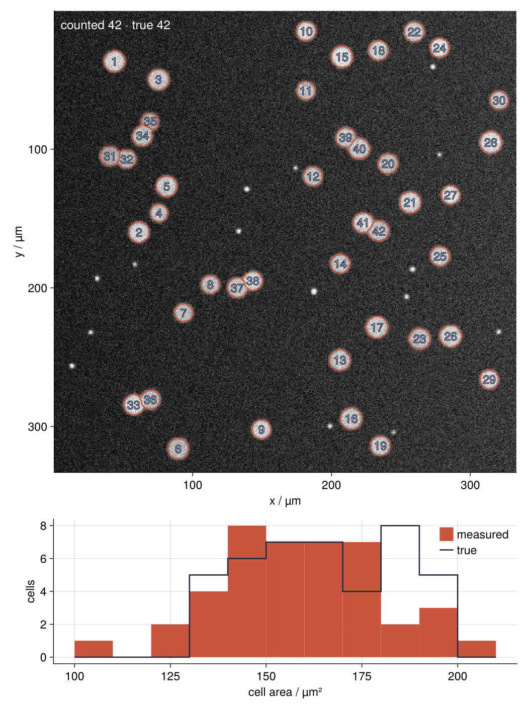
Every counted cell has its own outline and number, and the histogram sets the measured areas against the true ones. Step 6 draws it. Steps 1 to 4 smooth, threshold, label, and measure, and Step 5 splits the merged pairs. Before the split the count is 36; after it, 42 of 42, and the median cell measures 157 µm² where the truth is 165 µm². The image is synthetic so that every number has a truth to be checked against. The code does not care: a real micrograph with the same features runs through it unchanged, as do grains in a rock thin section or particles in an electron micrograph.

Setup

The cell below makes the synthetic image and keeps its truth, the centers and radii of the 42 cells, so that Step 6 can check the count. Run it without studying it: the method starts at Step 1. A seeded Xoshiro generator places the cells, six pairs overlapping, then adds debris, blur, background, and noise. The image img is a plain Matrix{Float64}, which every JuliaImages function below accepts as it is. rows and cols hold the row and column number of every pixel, counted from 1, so a disk is the condition (rows .- y).^2 .+ (cols .- x).^2 .<= r^2. The packages are loaded one by one, not through the Images umbrella package, which keeps the load time down. Install them once with import Pkg; Pkg.add(["ImageFiltering", "ImageMorphology", "ImageSegmentation", "CairoMakie"]); Random, Statistics, and Printf come with Julia.

using ImageFiltering, ImageMorphology, ImageSegmentation
using Random, Statistics, Printf
using CairoMakie

N = 512                        # image size in pixels
px = 0.65                      # µm per pixel: a 6.5 µm camera pixel behind a 10× objective
rng = Xoshiro(42)
rows = [i for i in 1:N, j in 1:N]
cols = [j for i in 1:N, j in 1:N]
uniform(a, b) = a + (b - a) * rand(rng)
indisk(c, r) = (rows .- c[1]).^2 .+ (cols .- c[2]).^2 .<= r^2   # true inside the disk at c = (row, column)

centers, radii, brightness = Vector{Float64}[], Float64[], Float64[]

# a cell at c with radius r keeps 4 px from the edge and 8 px from every other cell
free(c, r) = all(r + 4 .<= c .<= N - r - 4) &&
             all(hypot((c .- c2)...) >= r + r2 + 8 for (c2, r2) in zip(centers, radii))

function add!(c, r)
    push!(centers, c); push!(radii, r); push!(brightness, uniform(0.75, 1.0))
end

while length(centers) < 12                     # six touching pairs
    r1, r2 = uniform(10, 12.5), uniform(10, 12.5)
    c1 = [uniform(0, N), uniform(0, N)]
    angle = uniform(0, 2π)
    c2 = c1 .+ 0.85 * (r1 + r2) .* [cos(angle), sin(angle)]
    if free(c1, r1) && free(c2, r2)
        add!(c1, r1); add!(c2, r2)
    end
end
while length(centers) < 42                     # thirty single cells
    r = uniform(10, 12.5)
    c = [uniform(0, N), uniform(0, N)]
    free(c, r) && add!(c, r)
end

truth = zeros(N, N)
for (c, r, b) in zip(centers, radii, brightness)
    truth .= max.(truth, b .* indisk(c, r))
end
specks = Vector{Float64}[]
while length(specks) < 15                      # debris, at least 6 px from every cell
    r = uniform(1.5, 2.5)
    c = [uniform(r + 4, N - r - 4), uniform(r + 4, N - r - 4)]
    if all(hypot((c .- c2)...) >= r + r2 + 6 for (c2, r2) in zip(centers, radii))
        truth .= max.(truth, 2.5 .* indisk(c, r))
        push!(specks, c)
    end
end

img = imfilter(truth, Kernel.gaussian(1.5)) .+    # optical blur
      0.10 .+ 0.15 .* cols ./ N .+                 # background, brighter to the right
      0.1 .* randn(rng, N, N)                      # camera noise
n_true = length(radii)
true_area = π .* radii.^2 .* px^2                  # µm², for the check in Step 6

const INK, ACCENT, SECOND, MUTED = "#1f2a44", "#c8553d", "#2a7f9e", "#8a8f98"
set_theme!(Theme(
    size = (770, 396), fontsize = 17,
    palette = (color = [INK, ACCENT, SECOND, MUTED],),
    Axis = (topspinevisible = false, rightspinevisible = false, xgridvisible = true, ygridvisible = true),
    Lines = (linewidth = 2.5,),
))

# Makie puts an array's first index on x; an image has its rows running down. Every figure draws through this.
function showimage!(ax, A, rs, cs; colormap = :grays, colorrange = (0, 1.3))
    heatmap!(ax, cs .* px, rs .* px, permutedims(A[rs, cs]); colormap, colorrange)
    ax.yreversed = true
    ax.aspect = DataAspect()
end
# Outline every label of L inside the crop rs, cs with a contour at half height, one per label.
function outline!(ax, L, rs, cs; color = ACCENT, linewidth = 1.7)
    for k in setdiff(unique(L[rs, cs]), 0)
        contour!(ax, cs .* px, rs .* px, permutedims(Float64.(L[rs, cs] .== k)); levels = [0.5], color, linewidth)
    end
end

@printf("%d × %d pixels, %.2f µm per pixel, %d cells placed (6 touching pairs)\n", N, N, px, n_true)

512 × 512 pixels, 0.65 µm per pixel, 42 cells placed (6 touching pairs)

Step 1: Look at the image and smooth it with imfilter

Before anything else, ask the array for its size, its element type, and the span of its values:

println(size(img), " ", eltype(img))
@printf("brightness from %.2f to %.2f\n", extrema(img)...)

(512, 512) Float64
brightness from -0.32 to 2.01

The unit is arbitrary (a.u.). Negative values are noise riding on the dark background, and values near 2 are debris, about twice the brightness of a cell.

For a microscope file, with the packages FileIO and ImageIO, load("cells.tif") returns a 16-bit TIFF as a matrix of Gray{N0f16}, brightness stored in 16 bits and read as a fraction from 0 to 1. A file with several channels comes back with a third axis, and img[:, :, 1] takes the first. Convert with Float64.(img) before any arithmetic: the 16-bit fractions wrap around, so 0.1 minus 0.2 gives 0.9, and a subtracted background turns dark pixels bright.

imfilter sets each pixel to a weighted mean over its neighborhood, and the kernel is the table of weights. Kernel.gaussian(2) is a bell of weights with σ = 2 px, 1.3 µm, so the pixels within about 2 px count most. Noise differs from pixel to pixel and cancels in the average; anything wider than the kernel survives. The standard deviation std, the typical scatter around the mean, measures the noise in an empty corner:

smooth = imfilter(img, Kernel.gaussian(2))
corner = (N-49:N, N-49:N)
@printf("noise in an empty corner: %.3f raw, %.3f smoothed\n", std(img[corner...]), std(smooth[corner...]))

noise in an empty corner: 0.102 raw, 0.017 smoothed

Copy

rs, cs = 230:383, 150:303                      # a 100 µm square with a touching pair and two specks
fig = Figure(size = (770, 374))
for (i, (A, name)) in enumerate([(img, "raw"), (smooth, "σ = 2 px")])
    ax = Axis(fig[1, i], xlabel = "x / µm", ylabel = i == 1 ? "y / µm" : "",
              xgridvisible = false, ygridvisible = false)
    showimage!(ax, A, rs, cs)
    text!(ax, 0.04, 0.04; text = name, space = :relative, color = :white)
    i == 2 && hideydecorations!(ax, ticks = false)
end
fig

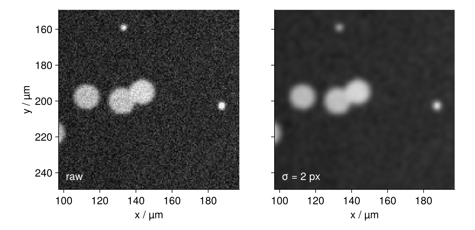
Smoothing cuts the noise sixfold and leaves the outlines of the pair and the specks intact. A wider kernel would soften the edges too, and where the edge sits decides the area. σ belongs well under the radius of the smallest thing you count.

Step 2: Read a threshold off the histogram and clean the mask

Every pixel brighter than some value counts as cell, and the brightness histogram tells you what that value should be. vec(smooth) lines the pixels up in one vector; the vertical axis is logarithmic, since background pixels vastly outnumber cell pixels:

Copy

fig = Figure(size = (770, 374))
ax = Axis(fig[1, 1], xlabel = "brightness / a.u.", ylabel = "pixels", yscale = log10)
hist!(ax, vec(smooth); bins = 200, color = INK, strokecolor = INK, strokewidth = 0.5, fillto = 0.5)   # fillto: bars start below 1 on the log axis
vlines!(ax, 0.6; color = SECOND, linestyle = :dash, linewidth = 1.4)
text!(ax, 0.62, 2e3; text = "threshold 0.6", color = SECOND)
ylims!(ax, 0.8, nothing)
fig

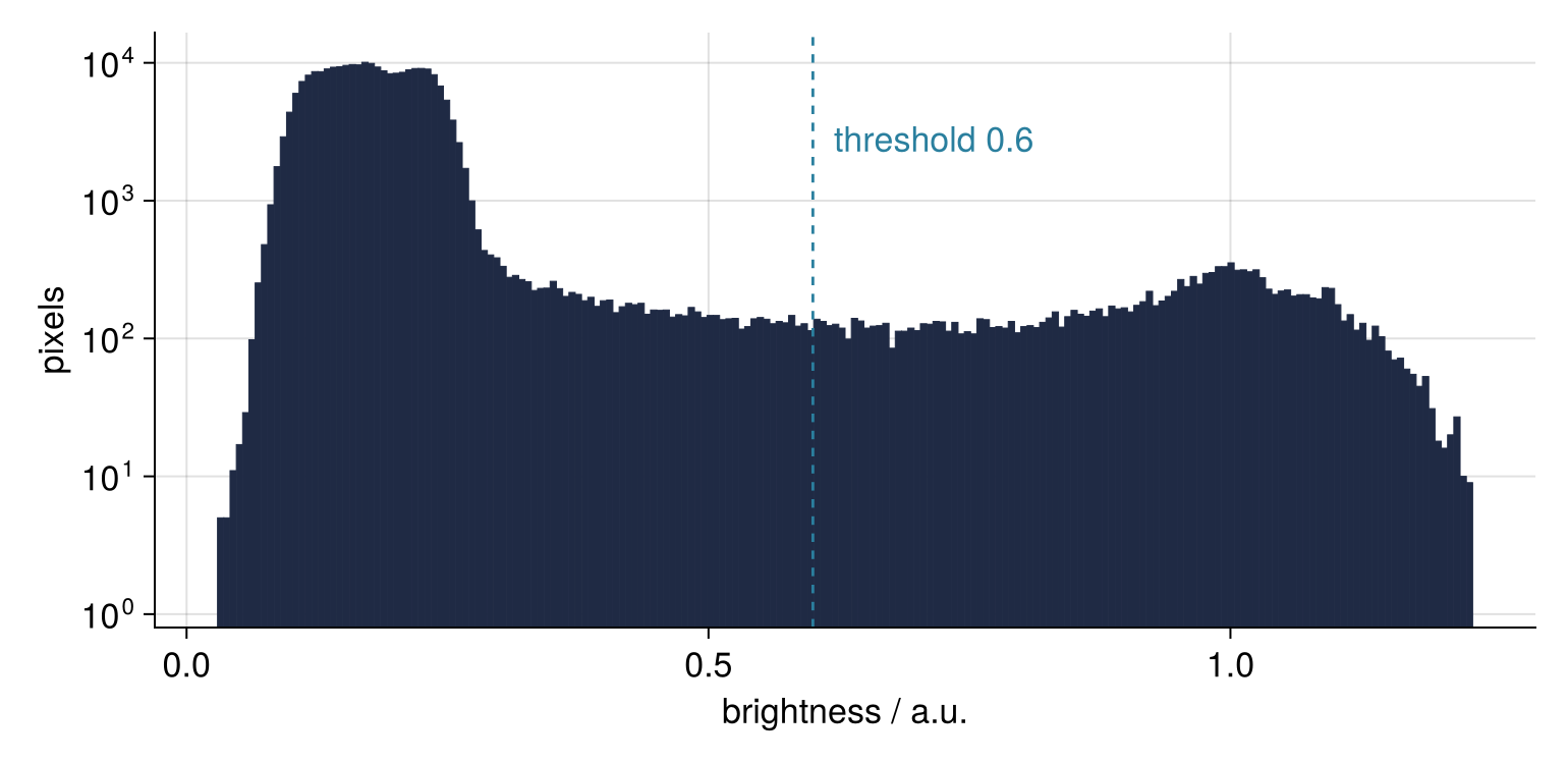
Background makes the tall peak between 0.1 and 0.3, cell interiors the low peak around 1.0, and cell edges the plateau in between. Put the threshold halfway between the peaks, 0.2 and 1.0: at 0.6. Blur smears the jump at a cell's edge into a slope, which on a straight edge passes half height exactly where the jump was. On a round edge it passes a fraction of a pixel inside, because more of the blur spills outward than inward. Step 6 prices that fraction.

smooth .> 0.6 gives a mask, true on cell pixels, and averaging trues and falses gives the share of trues:

raw_mask = smooth .> 0.6
@printf("cell pixels: %.1f %% of the image\n", 100 * mean(raw_mask))

cell pixels: 6.2 % of the image

Debris clears the threshold as well, but it is small. opening moves a small template, the structuring element, across the mask and keeps a true pixel only where some position of the template covers it while lying wholly inside the mask. With a disk of radius 4 px as template, a cell 20 px across survives almost untouched, and anything thinner than 9 px, 6 µm, disappears. centered renumbers the 9 × 9 table from -4 to 4, so that the middle of the disk sits at (0, 0). That is the form ImageMorphology expects; a plain 1-based table gives the same opening, because the package centers it itself, but that path is deprecated, and Julia hides the warning unless you start it with --depwarn=yes:

disk = centered([x^2 + y^2 <= 16 for y in -4:4, x in -4:4])
mask = opening(raw_mask, disk)
println(count(disk), " pixels in the disk")
Int.(disk)

49 pixels in the disk

9×9 OffsetArray(::Matrix{Int64}, -4:4, -4:4) with eltype Int64 with indices -4:4×-4:4:
 0  0  0  0  1  0  0  0  0
 0  0  1  1  1  1  1  0  0
 0  1  1  1  1  1  1  1  0
 0  1  1  1  1  1  1  1  0
 1  1  1  1  1  1  1  1  1
 0  1  1  1  1  1  1  1  0
 0  1  1  1  1  1  1  1  0
 0  0  1  1  1  1  1  0  0
 0  0  0  0  1  0  0  0  0

A rough circle of ones, numbered from -4 to 4 both ways.

Step 3: Label the connected regions with label_components

label_components hands out the numbers 1, 2, 3, and so on, one per connected region, writes each number into all pixels of its region, and leaves 0 on the background. Two pixels are connected when they share a side; a shared corner is not enough, a choice the second pitfall examines.

labels = label_components(mask)
n = maximum(labels)
println("regions without the opening: ", maximum(label_components(raw_mask)))
println("regions with the opening:    ", n)
println("cells in the image:          ", n_true)

regions without the opening: 51
regions with the opening:    36
cells in the image:          42

The opening took out 15 regions, one for each speck of debris, and no cell. The count still falls six short of 42, once for every touching pair.

Step 4: Measure each region with component_lengths and component_boxes

An area is a pixel count. component_lengths(labels) counts the pixels of every label, background included: index 0 holds the background and index k region k, so counts[1:n] are the regions. Times px^2, the area of one pixel, they are in µm²:

counts = component_lengths(labels)
area = counts[1:n] .* px^2
println(round.(Int, sort(area)))
@printf("median %.0f µm²\n", median(area))

[120, 130, 133, 135, 139, 145, 146, 146, 147, 148, 152, 154, 155, 156, 158, 161, 164, 169, 171, 174, 175, 176, 179, 180, 187, 188, 192, 194, 196, 208, 268, 277, 305, 312, 331, 333]
median 170 µm²

The first thirty areas climb steadily from 120 to 208 µm², and then the list leaps to 268. Thirty of the 36 regions are single cells, so the median, 170 µm², is the area of a typical cell. A merged pair, minus its overlap, comes out near twice that: the six regions past the leap are 1.6 to 2 times the median. A cut at 1.5 times the median sits halfway between one cell and two, and holds while no single cell reaches 1.5 times the typical one; the largest here is 1.2 times. If your cells vary more, find the gap in the sorted list by eye.

findall returns the numbers of the regions above the cut. The comprehension [l in merged for l in labels] runs over the label image and is true where a pixel belongs to one of them, an array of the image's shape. component_boxes gives the smallest rectangle around every region, numbered like counts, and the figure crops with it:

merged = findall(area .> 1.5 * median(area))
flagged = [l in merged for l in labels]
boxes = component_boxes(labels)
println("merged regions: labels ", merged)

merged regions: labels [1, 3, 5, 12, 20, 22]

Copy

s = maximum(maximum(length.(boxes[k].indices)) for k in merged) + 10   # one window size, 5 px margin
fig = Figure(size = (825, 187))
for (i, k) in enumerate(merged)
    r, c = boxes[k].indices
    r0 = clamp((first(r) + last(r) - s) ÷ 2, 1, N - s + 1)            # same scale in every crop
    c0 = clamp((first(c) + last(c) - s) ÷ 2, 1, N - s + 1)
    rs, cs = r0:r0+s-1, c0:c0+s-1
    ax = Axis(fig[2, i])
    showimage!(ax, img, rs, cs)
    contour!(ax, cs .* px, rs .* px, permutedims(Float64.(labels[rs, cs] .== k));
             levels = [0.5], color = SECOND, linewidth = 1.7)
    hidedecorations!(ax); hidespines!(ax)
    Label(fig[1, i], @sprintf("%.0f µm²", area[k]), tellwidth = false)
end
fig

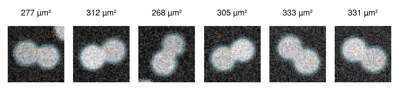
Every outline encloses two cells.

Step 5: Split touching cells with the distance transform and watershed

The hills. feature_transform points every pixel to the nearest true pixel of its argument, and distance_transform turns that into a distance. Given the background, .!mask, that is every cell pixel's distance to the background: one hill per cell, two with a saddle where a pair touches. Setup placed the pairs first, so cells 3 and 4 are one pair:

dist = distance_transform(feature_transform(.!mask))
p1, p2 = round.(Int, centers[3]), round.(Int, centers[4])
neck = (p1 .+ p2) .÷ 2
@printf("tops %.1f and %.1f px, neck %.1f px\n", dist[p1...], dist[p2...], dist[neck...])

tops 10.8 and 10.8 px, neck 8.5 px

Two tops of 10.8 px, the neck 2.3 px lower.

The markers. A marker is a seed from which one cell's label grows, one per hilltop. A pixel is a top when nothing in the w × w window around it is higher; mapwindow(maximum, dist, (w, w)) gives every pixel its window's maximum. .& flagged searches only the merged regions and so keeps out the background; dist .> 5 does that in the whole mask. Growing the tops by 3 px with dilate fuses the pixels of one top:

tops(w) = (dist .== mapwindow(maximum, dist, (w, w))) .& (dist .> 5) .& flagged
peaks = tops(15)
markers = label_components(dilate(peaks, strel_box((7, 7))))
for w in (5, 15, 25, 27)
    println("window $w × $w: ", maximum(label_components(tops(w))), " groups of top pixels")
end
println("markers after growing: ", maximum(markers))
@printf("closest centers of a pair: %.1f px\n", minimum(hypot((centers[k] .- centers[k+1])...) for k in 1:2:11))

window 5 × 5: 14 groups of top pixels
window 15 × 15: 12 groups of top pixels
window 25 × 25: 12 groups of top pixels
window 27 × 27: 10 groups of top pixels
markers after growing: 12
closest centers of a pair: 18.3 px

A 5 × 5 window also counts bumps on ragged edges. Too large, and the window around a pair's lower top reaches the higher one, so the lower top vanishes. A square reaches 0.7 w toward its corners, so keep 0.7 w under the closest spacing of two centers, 18.3 px: w under 26. At 27, two pairs lose a top. Anything in between works; we use 15. Growing changed nothing here; it is insurance against top pixels that meet only at a corner.

The split. watershed floods from the markers, lowest ground first, and draws a border where two floods meet. It wants valleys, so -dist turns every hill into a basin and the neck into a ridge. mask = flagged keeps the water inside the merged regions, and labels_map returns the labels, 0 outside. Lifted above n, the new labels cannot collide with the old ones; a lookup then renumbers everything 1 to K, so maximum(cells) is the count:

basins = labels_map(watershed(-dist, markers; mask = flagged))
cells = ifelse.(flagged, basins .+ n, labels)
used = sort(unique(cells))                                 # 0 first, then the labels in use
newnumber = Dict(l => k - 1 for (k, l) in enumerate(used)) # 0 stays 0
cells = [newnumber[l] for l in cells]
println("cells counted: ", maximum(cells))

cells counted: 42

Thirty-six regions, six split in two: 42.

Copy

rs, cs = 112:181, 296:365                      # one pair, 45 µm on a side
top = findall(peaks[rs, cs])                   # pixels of the two tops
fig = Figure(size = (770, 286))
panels = [(Float64.(mask), :grays, (0, 1)), (dist, :cividis, (0, 12)), (img, :grays, (0, 1.3))]
axs = [Axis(fig[1, i]) for i in 1:3]
for (ax, (A, cmap, crange), name) in zip(axs, panels, ["mask", "distance", "split"])
    showimage!(ax, A, rs, cs; colormap = cmap, colorrange = crange)
    hidedecorations!(ax); hidespines!(ax)
    text!(ax, 0.04, 0.05; text = name, space = :relative, color = :white)
end
scatter!(axs[2], [(cs[t[2]] * px, rs[t[1]] * px) for t in top]; color = ACCENT, markersize = 11)
outline!(axs[3], cells, rs, cs; linewidth = 2)
fig

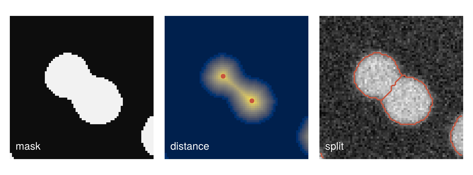
Mask, distance in cividis with the tops in red, and split: the border lies at the neck.

Step 6: Check the count and the sizes against the truth

Three comparisons with the truth: the count, the median area, and whether each true cell owns a label. For the last, argmax picks the label that most pixels of a true disk carry.

K = maximum(cells)
cell_area = component_lengths(cells)[1:K] .* px^2
@printf("counted %d, true %d\n", K, n_true)
@printf("median area %.0f µm², true %.0f µm² (%+.1f %%)\n", median(cell_area), median(true_area),
        100 * (median(cell_area) / median(true_area) - 1))

best = map(zip(centers, radii)) do (c, r)
    labs = cells[indisk(c, r)]
    argmax(l -> count(==(l), labs), unique(labs))   # the label most of its pixels carry
end
println(n_true, " true cells fall into ", length(unique(best)), " different labels")

counted 42, true 42
median area 157 µm², true 165 µm² (-5.2 %)
42 true cells fall into 42 different labels

Every cell is found, each in a label of its own. Areas come out 5.2 % small at the median, the price of a half-height threshold on round cells. The median also lies below Step 4's 170 µm², since six double regions are now twelve single cells. Sweep the threshold and you see how much more the size depends on it:

for t in (0.5, 0.6, 0.7, 0.8)
    lab = label_components(opening(smooth .> t, disk))
    k = maximum(lab)
    @printf("threshold %.1f: %d regions, median area %3.0f µm²\n", t, k, median(component_lengths(lab)[1:k] .* px^2))
end

threshold 0.5: 36 regions, median area 191 µm²
threshold 0.6: 36 regions, median area 170 µm²
threshold 0.7: 36 regions, median area 149 µm²
threshold 0.8: 36 regions, median area 127 µm²

The count holds at 36 from 0.5 to 0.8 and no speck survives, while the median area falls from 191 to 127 µm², about 21 µm² per step of 0.1, against 8 µm² between measured and true median. The threshold barely touches the count and sets the sizes.

Copy

centroids = component_centroids(cells)         # (row, column) of every label, index 0 the background
fig = Figure(size = (770, 1034))
ax = Axis(fig[1, 1], xlabel = "x / µm", ylabel = "y / µm", xgridvisible = false, ygridvisible = false)
showimage!(ax, img, 1:N, 1:N)
outline!(ax, cells, 1:N, 1:N)
text!(ax, [(c[2] * px, c[1] * px) for c in centroids[1:K]]; text = string.(1:K), align = (:center, :center),
      color = :white, strokecolor = INK, strokewidth = 1)
text!(ax, 5, 5; text = "counted $K · true $n_true", align = (:left, :top), color = :white, fontsize = 18)

ax_h = Axis(fig[2, 1], xlabel = "cell area / µm²", ylabel = "cells")
lo, hi = extrema(vcat(cell_area, true_area))
bins = floor(lo / 10) * 10 : 10 : hi + 10                        # 10 µm² bins, no empty ends
hist!(ax_h, cell_area; bins, color = ACCENT, label = "measured")
stephist!(ax_h, true_area; bins, color = INK, linewidth = 1.9, label = "true")
axislegend(ax_h; framevisible = false, position = :rt)
rowsize!(fig.layout, 2, Relative(2.2 / 9.2))
fig

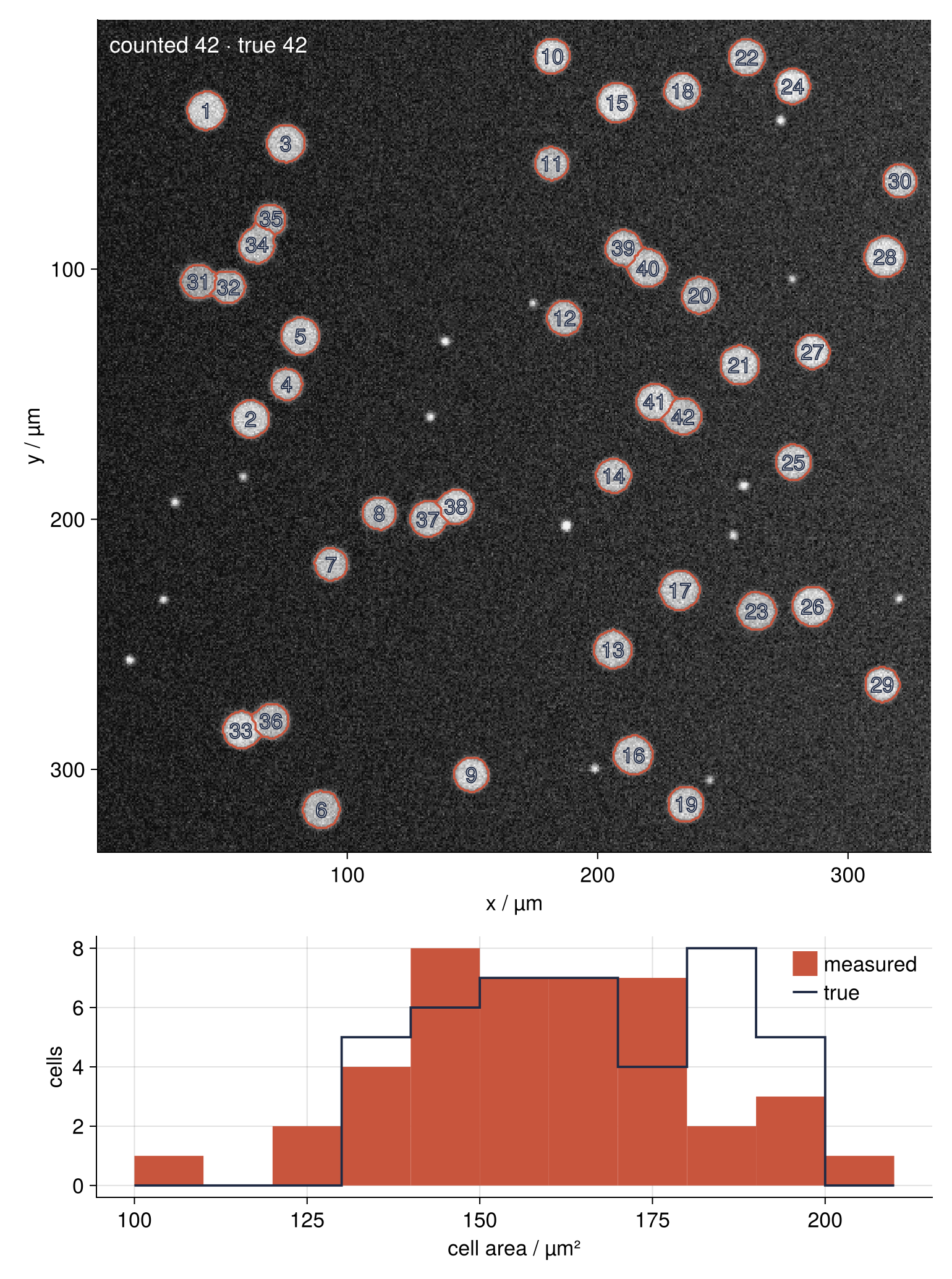
A real image comes without its truth, and four checks from this page replace it. Inspect the overlay one outline at a time. Pick a patch with 10 to 20 cells, count them yourself, and compare with the labels there. Scan the sorted areas: a region near twice the typical size is a pair the split missed, one near half of it a cell cut in two. Last, rerun at a few thresholds, and distrust any count that shifts.

Pitfalls

A global threshold under an uneven background. Make the background climb from 0.10 on the left to 0.85 on the right, where it reached 0.25 before, and 0.6 stops working:

smooth_steep = imfilter(img .+ 0.6 .* cols ./ N, Kernel.gaussian(2))
lab = label_components(opening(smooth_steep .> 0.6, disk))
k = maximum(lab)
@printf("global threshold: %.0f %% of pixels are cell, %d regions, largest %.0f µm²\n",
        100 * mean(lab .> 0), k, maximum(component_lengths(lab)[1:k]) * px^2)

flat = tophat(smooth_steep, strel_box((41, 41)))
println("after tophat: ", maximum(label_components(opening(flat .> 0.4, disk))), " regions")

global threshold: 38 % of pixels are cell, 22 regions, largest 37030 µm²
after tophat: 36 regions

Now 38 % of the image passes as cell, the right side merges into one region of 37,030 µm², a third of the field, and the count drops to 22. No single number separates cells from a background that crosses it, so subtract an estimate of the background first. tophat makes that estimate by opening the brightness values with a 41 × 41 box. Pass one gives every pixel the minimum over its box; no cell, at most 25 px wide, fills the box, so the minimum near a cell is background and the cells are gone. Pass two gives every pixel the maximum over its box, which restores the gentle slope and nothing else. tophat subtracts this estimate and leaves the cells standing on a flat zero, so the half-height threshold drops to 0.4, half of what a cell reaches. With it the count returns to 36. Choose a box larger than your largest object.

label_components connects only four neighbors. Unless told otherwise, it links a pixel to the four pixels that share a side with it, never to the four diagonal ones. A diagonal line falls apart pixel by pixel; strel_box((3, 3)), a 3 × 3 block, connects all eight neighbors:

line = [i == j for i in 1:5, j in 1:5]
println("diagonal line: ", maximum(label_components(line)), " regions by default, ",
        maximum(label_components(line, strel_box((3, 3)))), " with eight neighbors")
println("cells of Step 3 with eight neighbors: ", maximum(label_components(mask, strel_box((3, 3)))))

diagonal line: 5 regions by default, 1 with eight neighbors
cells of Step 3 with eight neighbors: 36

Round cells do not notice: 36 regions both ways. Fibers and cracks that run at an angle do, and the default shatters each of them. Always pass strel_box((3, 3)); round objects lose nothing by it, and slanted thin ones stay in one piece.

Areas in pixels, or in the wrong unit. component_lengths counts pixels; µm² need the square of the pixel size, px^2. Multiply by px once and every area comes out 1/0.65 = 1.54 times too large. The pixel size follows from the optics, a 6.5 µm sensor pixel behind a 10× objective giving 0.65 µm, and 2 × 2 binning makes it twice that. Take it from the file's metadata; a remembered value belongs to last year's camera.

Variations

• Brightness per cell. Loop once over the pixels, add img[i] to the sum of label cells[i] and 1 to its count, and divide: the mean fluorescence per cell, which is what an expression study measures next. Remove the background beforehand with tophat, as in the first pitfall.
• Mineral grains in a thin section. In rock nearly every grain borders others, so skip the size flag, look for tops in the whole mask, flood with mask = mask, and report the equivalent diameter 2 .* sqrt.(area ./ π). The height cut dist .> 5 then earns its place by keeping the background out of the markers.
• Particles in an electron micrograph. A particle cut by the image edge comes out too small. Drop every label whose component_boxes rectangle touches row or column 1 or N.
• The split without watershed. feature_transform(markers .> 0) gives each pixel the position of its nearest marker pixel, and indexing markers with it gives that marker's number. It is cheaper, and it cuts along the straight line midway between two markers instead of the neck.

Cheat sheet

smooth = imfilter(Float64.(img), Kernel.gaussian(2))            # Float64 first; σ well below the smallest radius
flat = tophat(smooth, strel_box((41, 41)))                      # box wider than the largest object
mask = opening(flat .> t, centered([x^2 + y^2 <= 16 for y in -4:4, x in -4:4]))   # t at half height
labels = label_components(mask, strel_box((3, 3)))              # eight neighbors; count before splitting
dist = distance_transform(feature_transform(.!mask))            # a hill per object
peaks = (dist .== mapwindow(maximum, dist, (w, w))) .& (dist .> h)   # 0.7 w < closest center spacing, h = r_min / 2
markers = label_components(dilate(peaks, strel_box((7, 7))))    # fuse the pixels of one top
cells = labels_map(watershed(-dist, markers; mask))             # split every object along its neck
area = component_lengths(cells)[1:maximum(cells)] .* px^2       # µm²; index 0 is the background

Further reading

• The JuliaImages documentation, with the reference pages of ImageFiltering, ImageMorphology, and ImageSegmentation.
• Pete Bankhead's Introduction to Bioimage Analysis, free online, explains thresholds, morphology, and measurement with biological images in mind. Gonzalez and Woods, Digital Image Processing, is the standard textbook on the methods.
• On this site: Counting cells with scipy.ndimage: how many are there, and how large?, this tutorial in Python; DataFrames.jl from the ground up: a week of temperature logs, to put the per-cell areas in a table; and The Fourier transform in Julia: asking a signal how much of each frequency it contains, for what a Gaussian smoothing does to frequencies.
• Download the notebook. It was executed with the library versions in the header.