Counting cells with scipy.ndimage: how many are there, and how large?

The problem: how many cells, and how large?

Here is a fluorescence image of cultured cells, 512 × 512 pixels at 0.65 µm per pixel, so a field 333 µm wide. The cells are bright round blobs 13 to 16 µm across on a dark background that brightens from left to right, with camera noise over everything and a few specks of bright debris. You want two answers: how many cells there are, and how large each one is. scipy.ndimage gives both in four operations: smooth, threshold, label, measure.

Those four alone get the count wrong, and always in the same direction. Where two cells touch, the threshold sees one bright region, so every touching pair is counted as one cell. A fifth operation, built on the distance from each cell pixel to the background, splits the pairs again.

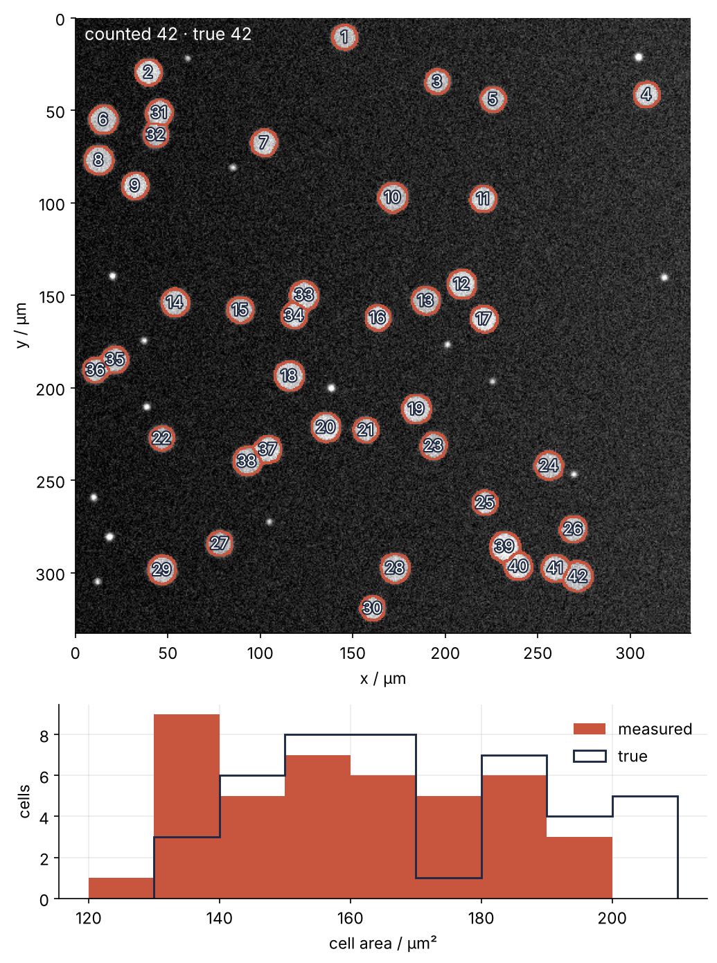
Synthetic fluorescence image of 42 cells, each outlined in red and numbered; touching pairs are split into two outlines. Below: histogram of measured cell areas in square micrometers, with the true areas as an outline.

Steps 1 to 4 do the four operations, Step 5 splits the merged pairs, and Step 6 draws the outlines and the histogram. The first count is 36. After the split it is 42 of 42, with a median area of 157 µm² against a true 164 µm². The image is synthetic so that the count can be checked against the truth. A real image with the same features goes through the same code, and so do mineral grains in a thin section or particles in an electron micrograph.

Setup

The image is a NumPy array of brightness values, one number per pixel, and ndi is the usual short name for scipy.ndimage. The cell below places 42 disks at random, six pairs of them overlapping, then adds debris, blur, background, and noise, and keeps the true positions and sizes for the check at the end. You need not study it; the seeded generator is the subject of Random numbers with numpy.random.

import numpy as np
import matplotlib.pyplot as plt
import matplotlib.patheffects as pe
from matplotlib.colors import to_rgba
from scipy import ndimage as ndi

N = 512                        # image size in pixels
px = 0.65                      # µm per pixel: a 6.5 µm camera pixel behind a 10× objective
rng = np.random.default_rng(42)
rows, cols = np.indices((N, N))    # row and column number of every pixel

centers, radii, brightness = [], [], []

def free(c, r):
    """True if a cell at c with radius r keeps 4 px from the edge and 8 px from every other cell."""
    inside = np.all((c >= r + 4) & (c <= N - r - 4))
    return inside and all(np.hypot(*(c - c2)) >= r + r2 + 8 for c2, r2 in zip(centers, radii))

def add(c, r):
    centers.append(c)
    radii.append(r)
    brightness.append(rng.uniform(0.75, 1.0))

while len(centers) < 12:                       # six touching pairs
    r1, r2 = rng.uniform(10, 12.5, 2)
    c1 = rng.uniform(0, N, 2)
    angle = rng.uniform(0, 2 * np.pi)
    c2 = c1 + 0.85 * (r1 + r2) * np.array([np.cos(angle), np.sin(angle)])
    if free(c1, r1) and free(c2, r2):
        add(c1, r1)
        add(c2, r2)
while len(centers) < 42:                       # thirty single cells
    r = rng.uniform(10, 12.5)
    c = rng.uniform(0, N, 2)
    if free(c, r):
        add(c, r)
centers, radii = np.array(centers), np.array(radii)

truth = np.zeros((N, N))
for (cy, cx), r, b in zip(centers, radii, brightness):
    truth = np.maximum(truth, b * ((rows - cy)**2 + (cols - cx)**2 <= r**2))

specks = []
while len(specks) < 15:                        # debris, at least 6 px from every cell
    r = rng.uniform(1.5, 2.5)
    c = rng.uniform(r + 4, N - r - 4, 2)
    if np.all(np.hypot(*(centers - c).T) >= radii + r + 6):
        truth = np.maximum(truth, 2.5 * ((rows - c[0])**2 + (cols - c[1])**2 <= r**2))
        specks.append(c)

image = (ndi.gaussian_filter(truth, 1.5)       # optical blur
         + 0.10 + 0.15 * cols / N              # background, brighter to the right
         + rng.normal(0, 0.1, (N, N)))         # camera noise
n_true = len(radii)
true_area = np.pi * radii**2 * px**2           # µm², for the check in Step 6

plt.rcParams.update({
    "figure.figsize": (7, 3.6), "figure.dpi": 110,
    "axes.spines.top": False, "axes.spines.right": False,
    "axes.grid": True, "grid.alpha": 0.25,
    "font.size": 11, "lines.linewidth": 1.8,
})
INK, ACCENT, SECOND, MUTED = "#1f2a44", "#c8553d", "#2a7f9e", "#8a8f98"

print(f"{N} × {N} pixels, {px} µm per pixel, {n_true} cells placed (6 touching pairs)")

512 × 512 pixels, 0.65 µm per pixel, 42 cells placed (6 touching pairs)

Step 1: Look at the image and smooth it with gaussian_filter

An image is an array with a shape, a data type, and a range of values:

print(image.shape, image.dtype)
print(f"brightness from {image.min():.2f} to {image.max():.2f}")

(512, 512) float64
brightness from -0.33 to 2.09

Brightness is in arbitrary units (a.u.), as it is for most cameras until someone calibrates them. Below zero is noise on the dark background; near 2 is debris, brighter than any cell.

This array is float64 because the generator made it so. A microscope file usually is not. tifffile.imread("cells.tif"), from the package tifffile (pip install tifffile), returns a TIFF as a NumPy array, often of type uint16, with one more axis if the file holds several channels: shape (2, 512, 512) for two. Take the channel that shows the cells, img[0] when the channels come first or img[..., 0] when they come last (... stands for all the axes before it), and convert it with .astype(float). On integers gaussian_filter rounds every average to a whole number, and a subtracted background wraps around to values near 65,535 instead of going below zero.

ndi.gaussian_filter replaces each pixel by a weighted average of its neighbors, with weights that fall off as a bell curve of width sigma pixels. Take sigma=2, 1.3 µm, a tenth of a cell diameter. To see what it does, measure the noise in an empty corner, image[-50:, -50:] (the last 50 rows and columns), as the standard deviation .std(): how far the values scatter around their mean.

smooth = ndi.gaussian_filter(image, sigma=2)
print(f"noise in an empty corner: {image[-50:, -50:].std():.3f} raw, {smooth[-50:, -50:].std():.3f} smoothed")

noise in an empty corner: 0.099 raw, 0.014 smoothed

r0, c0, w = 210, 0, 154                        # a 100 µm square on the left edge
extent = [c0 * px, (c0 + w) * px, (r0 + w) * px, r0 * px]
fig, axes = plt.subplots(1, 2, figsize=(7, 3.4), sharey=True)
for ax, img, name in zip(axes, [image, smooth], ["raw", "sigma = 2 px"]):
    ax.imshow(img[r0:r0 + w, c0:c0 + w], cmap="gray", vmin=0, vmax=1.3, extent=extent)
    ax.text(0.03, 0.04, name, color="white", transform=ax.transAxes)
    ax.set(xlabel="x / µm")
    ax.grid(False)
axes[0].set(ylabel="y / µm")
plt.show()

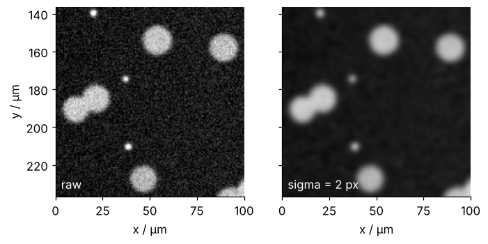
The noise falls by a factor of seven, and the touching pair and the specks keep their shape. A larger sigma removes more noise and blurs the edges more, and the edge decides the area. Keep sigma well below the radius of the smallest object you want to count.

Step 2: Read a threshold off the histogram and clean the mask

A threshold splits the pixels into cell and not cell. To choose it, look at the histogram of brightness. .ravel() lays the 512 × 512 values out in one row, and the count axis is logarithmic because background pixels far outnumber cell pixels:

fig, ax = plt.subplots(figsize=(7, 3.4))
ax.hist(smooth.ravel(), bins=200, color=INK)
ax.set_axisbelow(True)                         # grid behind the bars
ax.axvline(0.6, color=SECOND, ls="--", lw=1)
ax.text(0.62, 2e3, "threshold 0.6", color=SECOND)
ax.set(xlabel="brightness / a.u.", ylabel="pixels", yscale="log")
plt.show()

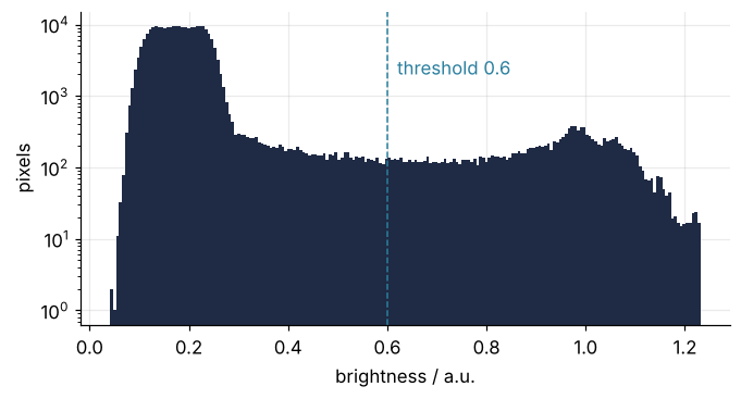
The tall hump from 0.1 to 0.3 is background, the low one around 1.0 is the inside of the cells, and the flat stretch between them is cell edges. Put the threshold halfway between the background, about 0.2, and the cells, about 1.0: 0.6. Blur turns the sharp step at a cell's edge into a ramp. On a straight edge the ramp passes its halfway point exactly where the step was. On a round cell it passes a fraction of a pixel inside, because at the edge more of the blur's weight falls outside the disk than in it. A half-height threshold puts the edge back to within that fraction, and Step 6 shows what it costs in area.

smooth > 0.6 is a mask, True on cell pixels, and the mean of True and False values is the fraction that is True:

raw_mask = smooth > 0.6
print(f"cell pixels: {100 * raw_mask.mean():.1f} % of the image")

cell pixels: 6.2 % of the image

The debris passes too, and its size gives it away. ndi.binary_opening slides a small shape, the structuring element, over the mask and keeps only the parts that the shape fits into completely. A disk of radius 4 px leaves round cells 20 px across nearly unchanged and removes anything narrower than 9 px (6 µm). np.mgrid[-4:5, -4:5] gives a 9 × 9 grid of row and column offsets from the center, and the disk keeps those within 4 px:

yy, xx = np.mgrid[-4:5, -4:5]
disk = xx**2 + yy**2 <= 16
mask = ndi.binary_opening(raw_mask, structure=disk)
print(disk.astype(int))

[[0 0 0 0 1 0 0 0 0]
 [0 0 1 1 1 1 1 0 0]
 [0 1 1 1 1 1 1 1 0]
 [0 1 1 1 1 1 1 1 0]
 [1 1 1 1 1 1 1 1 1]
 [0 1 1 1 1 1 1 1 0]
 [0 1 1 1 1 1 1 1 0]
 [0 0 1 1 1 1 1 0 0]
 [0 0 0 0 1 0 0 0 0]]

Printed as ones and zeros, the disk is a rough circle of 49 pixels.

Step 3: Label the connected regions and count them

ndi.label gives the pixels of each connected region of the mask the same integer, numbers the regions 1 to n, and leaves the background at 0. Connected means sharing an edge, which the second pitfall comes back to.

labels, n = ndi.label(mask)
print(f"regions without the opening: {ndi.label(raw_mask)[1]}")
print(f"regions with the opening:    {n}")
print(f"cells in the image:          {n_true}")

regions without the opening: 49
regions with the opening:    36
cells in the image:          42

The 13 regions the opening removed are debris; the other two of the 15 specks were already smoothed below the threshold. The six missing cells are the touching pairs, each counted once.

Step 4: Measure each region with sum_labels and find_objects

An area is a pixel count. ndi.sum_labels adds up an array over each region, so on np.ones_like(image), an array of ones the size of the image, it counts pixels. np.arange(1, n + 1) lists the labels 1 to 36, and px**2, the area of one pixel, turns pixels into µm²:

ids = np.arange(1, n + 1)
area = ndi.sum_labels(np.ones_like(image), labels, index=ids) * px**2
print(np.sort(area).round().astype(int))
print(f"median {np.median(area):.0f} µm²")

[127 131 132 133 136 136 137 137 141 145 150 152 152 154 154 156 158 160
 166 174 174 176 176 183 184 188 188 188 189 193 283 285 317 333 357 358]
median 163 µm²

Thirty regions lie between 127 and 193 µm², then the list jumps to 283. The six above the jump, about twice the median of 163 µm², are the merged pairs, and a cut at 1.5 times the median catches all six. That works because the single cells here vary in area by less than a factor of 1.6. With a wider spread, read the gap off the sorted list instead.

np.isin asks, pixel by pixel, whether a value is in a list, so flagged is True on every pixel of a merged region. ndi.find_objects returns the smallest rectangle around each region as a pair of slices, and image[boxes[k - 1]] crops region k (the list starts at label 1, Python at 0).

big = ids[area > 1.5 * np.median(area)]
flagged = np.isin(labels, big)
boxes = ndi.find_objects(labels)
print(f"merged regions: labels {big}")

merged regions: labels [ 6 14 20 27 32 35]

fig, axes = plt.subplots(1, 6, figsize=(7.5, 1.7))
s = max(sl.stop - sl.start for k in big for sl in boxes[k - 1]) + 10   # one window size, 5 px margin
for ax, k in zip(axes, big):
    r, c = boxes[k - 1]
    r0 = min(max((r.start + r.stop - s) // 2, 0), N - s)   # same scale in every crop
    c0 = min(max((c.start + c.stop - s) // 2, 0), N - s)
    crop = np.s_[r0:r0 + s, c0:c0 + s]
    ax.imshow(image[crop], cmap="gray", vmin=0, vmax=1.3)
    ax.contour(labels[crop] == k, levels=[0.5], colors=SECOND, linewidths=1.2)
    ax.text(0.5, 1.04, f"{area[k - 1]:.0f} µm²", ha="center", transform=ax.transAxes)
    ax.set_axis_off()
plt.show()

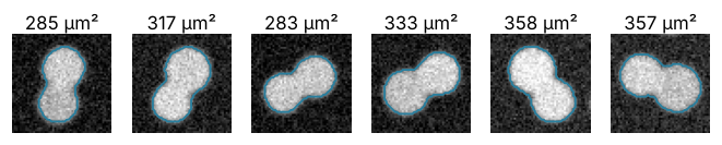
Each crop, 34 µm on a side, holds two cells inside one outline.

Step 5: Split touching cells with the distance transform

The hills. ndi.distance_transform_edt(mask) gives every cell pixel its distance to the nearest background pixel. A round cell becomes a hill topped at its center, and a touching pair two hills with a saddle at the neck. One pair, at its centers and halfway between:

dist = ndi.distance_transform_edt(mask)
(y1, x1), (y2, x2) = centers[2:4].round().astype(int)     # a pair: Setup placed the pairs first
print(f"tops {dist[y1, x1]:.1f} and {dist[y2, x2]:.1f} px, neck {dist[(y1 + y2) // 2, (x1 + x2) // 2]:.1f} px")

tops 11.7 and 9.4 px, neck 7.6 px

Tops of 11.7 and 9.4 px, saddle 7.6 px.

The markers. A marker is a seed for one cell, here a hilltop, and on a pixel grid a top can be two pixels of equal height, sometimes touching only at a corner. ndi.maximum_filter(dist, size=15) replaces every pixel by the largest value in the 15 × 15 window around it, so a pixel equal to that is a top. The window must be narrower than a pair's center spacing, 17 px or more here, or one top hides the other. dist > 5, half the smallest radius, drops low bumps on the rim, and & flagged keeps the merged regions. Growing every top by 3 px with binary_dilation fuses its pixels:

peaks = (dist == ndi.maximum_filter(dist, size=15)) & (dist > 5) & flagged
markers, n_markers = ndi.label(ndi.binary_dilation(peaks, iterations=3))
print(f"groups of top pixels: {ndi.label(peaks)[1]}, markers after growing: {n_markers}")

groups of top pixels: 13, markers after growing: 12

Thirteen groups became 12 markers: one top was two pixels touching at a corner, which label keeps apart (the second pitfall).

The split. Each pixel of a merged region now goes to its nearest marker, which the distance transform finds with the two sides swapped. Above, it measured from each cell pixel to the nearest zero of mask; on markers == 0 the zeros are the markers. return_indices=True adds where the nearest zero lies, as row and column arrays iy, ix, so markers[iy, ix] is that marker's number.

_, (iy, ix) = ndi.distance_transform_edt(markers == 0, return_indices=True)   # _: the distances
cells = np.where(flagged, markers[iy, ix] + n, labels)   # flagged: marker + n (clear of 1 to n), else old label
_, cells = np.unique(cells, return_inverse=True)         # renumber without gaps; 0 stays 0, shape stays
print(f"cells counted: {cells.max()}")

cells counted: 42

Thirty-six regions, six of them split in two: 42.

r0, c0, w = 204, 151, 70                       # one pair, 45 µm on a side
crop = np.s_[r0:r0 + w, c0:c0 + w]
ty, tx = np.nonzero(peaks[crop])               # pixels of the two tops
outline = np.zeros((w, w, 4))
outline[ndi.morphological_gradient(cells[crop], size=3) > 0] = to_rgba(ACCENT)   # where the label changes
fig, axes = plt.subplots(1, 3, figsize=(7, 2.6))
axes[0].imshow(mask[crop], cmap="gray")
axes[1].imshow(dist[crop], cmap="cividis")
axes[1].plot(tx, ty, "o", color=ACCENT, ms=4)
axes[2].imshow(image[crop], cmap="gray", vmin=0, vmax=1.3)
axes[2].imshow(outline, interpolation="none")
for ax, name in zip(axes, ["mask", "distance", "split"]):
    ax.text(0.04, 0.05, name, color="white", transform=ax.transAxes)
    ax.set_axis_off()
plt.show()

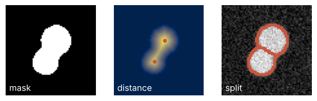
The pair, 45 µm on a side, as mask, as distance map (cividis) with its tops in red, and split. The cut is a straight line halfway between the markers: enough for counting, while the watershed in the last variation follows the neck.

Step 6: Check the count and the sizes against the truth

Compare count and median area with the truth, and check that each true cell got its own label: np.bincount counts the label numbers among a true cell's pixels, and argmax picks the most frequent.

cell_area = ndi.sum_labels(np.ones_like(image), cells, np.arange(1, cells.max() + 1)) * px**2
print(f"counted {cells.max()}, true {n_true}")
print(f"median area {np.median(cell_area):.0f} µm², true {np.median(true_area):.0f} µm²")

best = []
for (cy, cx), r in zip(centers, radii):
    inside = (rows - cy)**2 + (cols - cx)**2 <= r**2       # pixels of one true cell
    best.append(np.bincount(cells[inside]).argmax())       # the label most of them carry
print(f"{n_true} true cells fall into {len(set(best))} different labels")

counted 42, true 42
median area 157 µm², true 164 µm²
42 true cells fall into 42 different labels

The count is right and no label holds two cells. The median area is 4 % low, the cost of Step 2's half-height threshold on round cells: a fraction of a pixel on a radius of 10 to 12.5 px is a few percent of the area. It is also below Step 4's 163 µm², because six double-size regions are now twelve cells of normal size. A sweep over the threshold shows how much more the size depends on where you put it:

for t in [0.5, 0.6, 0.7, 0.8]:
    lab, k = ndi.label(ndi.binary_opening(smooth > t, structure=disk))
    a = ndi.sum_labels(np.ones_like(image), lab, np.arange(1, k + 1)) * px**2
    print(f"threshold {t:.1f}: {k} regions, median area {np.median(a):3.0f} µm²")

threshold 0.5: 37 regions, median area 182 µm²
threshold 0.6: 36 regions, median area 163 µm²
threshold 0.7: 36 regions, median area 142 µm²
threshold 0.8: 36 regions, median area 123 µm²

From 0.6 to 0.8 the count stays at 36 while the median area falls from 163 to 123 µm². At 0.5 a speck on the bright side grows wide enough to survive the opening. The count holds and the size moves with the edge, by about 20 µm² per step of 0.1, against the 7 µm² that half height costs. A size distribution is only as good as its threshold.

ids_final = np.arange(1, cells.max() + 1)
overlay = np.zeros((N, N, 4))
overlay[ndi.morphological_gradient(cells, size=3) > 0] = to_rgba(ACCENT)
# center of mass of a label: the mean position of its pixels
centers_found = ndi.center_of_mass(np.ones_like(image), cells, ids_final)

fig, (ax, ax_h) = plt.subplots(2, 1, figsize=(7, 9.4), height_ratios=[7, 2.2])
full = [0, N * px, N * px, 0]
ax.imshow(image, cmap="gray", vmin=0, vmax=1.3, extent=full)
ax.imshow(overlay, extent=full, interpolation="none")
for k, (y, x) in zip(ids_final, centers_found):
    ax.text(x * px, y * px, str(k), color="white", ha="center", va="center",
            path_effects=[pe.withStroke(linewidth=2, foreground=INK)])
ax.text(5, 12, f"counted {cells.max()} · true {n_true}", color="white", fontsize=12)
ax.set(xlabel="x / µm", ylabel="y / µm")
ax.grid(False)

both = np.concatenate([cell_area, true_area])
bins = np.arange(np.floor(both.min() / 10) * 10, both.max() + 10, 10)   # 10 µm² bins, no empty ends
ax_h.set_axisbelow(True)
ax_h.hist(cell_area, bins=bins, color=ACCENT, label="measured")
ax_h.hist(true_area, bins=bins, histtype="step", color=INK, lw=1.4, label="true")
ax_h.set(xlabel="cell area / µm²", ylabel="cells")
ax_h.legend(frameon=False, loc="upper right")
fig.tight_layout()
plt.show()

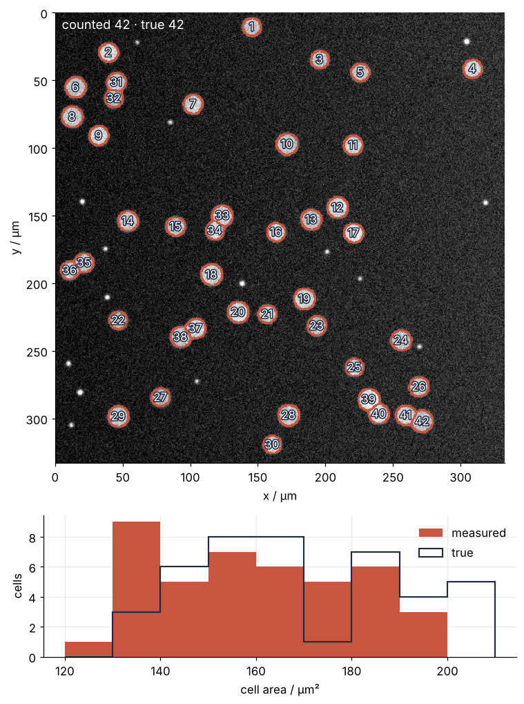
On your own image there is no truth to compare against, and four checks stand in for it. Look at the outline overlay cell by cell. Count one crop of 10 to 20 cells by hand, about 200 × 200 µm here, and compare with the labels in that crop. Read the sorted area list of Step 4, where a double-size outlier is a missed split and a half-size one a false split. And sweep the threshold: a count that moves with it is not to be trusted.

Pitfalls

A global threshold under an uneven background. Make the background rise from 0.10 to 0.85 across the field instead of to 0.25, and the same threshold of 0.6 gives up:

smooth_steep = ndi.gaussian_filter(image + 0.6 * cols / N, sigma=2)
lab, k = ndi.label(ndi.binary_opening(smooth_steep > 0.6, structure=disk))
largest = ndi.sum_labels(np.ones_like(image), lab, np.arange(1, k + 1)).max() * px**2
print(f"global threshold: {100 * (lab > 0).mean():.0f} % of pixels are cell, {k} regions, largest {largest:.0f} µm²")

flat = ndi.white_tophat(smooth_steep, size=41)
lab, k = ndi.label(ndi.binary_opening(flat > 0.4, structure=disk))
print(f"after white_tophat: {k} regions")

global threshold: 39 % of pixels are cell, 32 regions, largest 37045 µm²
after white_tophat: 36 regions

With one threshold, 39 % of the pixels count as cell, the bright side of the field becomes one region of 37,045 µm², a third of the image, and the count drops to 32. One number cannot separate cell from background when the background crosses it. Subtract a background estimate first. white_tophat makes the estimate with an opening on brightness values, two passes of a 41 × 41 px window. The first sets each pixel to the darkest value in its window; a cell, 25 px across at most, cannot fill the window, so the darkest value near a cell is background and the cells vanish. The second sets each pixel to the brightest value in its window, which rebuilds the slow rise across the field but not the cells. What remains is the image without its cells, and white_tophat returns the image minus that: cells on a flat zero. The half-height threshold is now half the cell brightness, 0.4, not Step 2's 0.6. The count is back at 36. The window must be wider than the largest object.

label connects only four neighbors. In 2D the default connects a pixel to its left, right, upper, and lower neighbors, not to its diagonal ones. A diagonal line, np.eye(5) (a 5 × 5 array with ones on the diagonal), falls apart into five pieces; structure=np.ones((3, 3)), a 3 × 3 block of ones, counts all eight neighbors:

line = np.eye(5)
print(f"diagonal line: {ndi.label(line)[1]} regions by default, "
      f"{ndi.label(line, structure=np.ones((3, 3)))[1]} with eight neighbors")
print(f"cells of Step 3 with eight neighbors: {ndi.label(mask, structure=np.ones((3, 3)))[1]}")

diagonal line: 5 regions by default, 1 with eight neighbors
cells of Step 3 with eight neighbors: 36

For round cells it changes nothing. For thin, diagonal objects such as fibers or cracks it splits one object into many. Pass structure=np.ones((3, 3)) every time: it costs nothing on round objects and keeps thin ones whole.

Areas in pixels, or in the wrong unit. sum_labels counts pixels. Multiply by px**2, not by px: forgetting the square makes every area 1/0.65 = 1.54 times too large here. The pixel size is the camera pixel divided by the magnification, 6.5 µm / 10 = 0.65 µm, and 2 × 2 binning doubles it. Take it from the image's metadata, not from memory.

Variations

Brightness per cell. ndi.mean(image, cells, ids_final) gives the mean fluorescence of every cell, the number an expression experiment needs next. Subtract the background first, as in the first pitfall.
Mineral grains in a thin section. Grains touch their neighbors almost everywhere, so drop the size flag and split every region as in Step 5. Report the equivalent diameter, 2 * np.sqrt(area / np.pi), for a grain-size distribution.
Particles in an electron micrograph. Particles cut by the image edge bias the sizes downward. Drop every label whose find_objects box starts at row or column 0 or ends at N.
scikit-image, the next step. skimage.filters.threshold_otsu picks the threshold from the histogram, skimage.segmentation.watershed(-dist, markers, mask=mask) floods the distance map from the markers and cuts along the neck instead of a straight line, and skimage.measure.regionprops_table returns area, eccentricity, and intensity as a table. SciPy's own ndi.watershed_ift looks like the same tool, but it charges a path only for its steepest step between neighboring pixels, so on a smooth distance map such as this one every path is cheap and one marker takes most of each pair.

Cheat sheet

smooth = ndi.gaussian_filter(img.astype(float), sigma=2)      # float first; sigma well below the smallest radius
flat = ndi.white_tophat(smooth, size=41)                       # window wider than the largest object
mask = ndi.binary_opening(flat > t, structure=disk)            # t at half height; disk from np.mgrid
labels, n = ndi.label(mask, structure=np.ones((3, 3)))         # count before splitting; eight neighbors
dist = ndi.distance_transform_edt(mask)                        # a hill per object
peaks = (dist == ndi.maximum_filter(dist, size=w)) & (dist > h)   # w < spacing, h = r_min / 2
markers, m = ndi.label(ndi.binary_dilation(peaks, iterations=3))  # fuse the pixels of one top
_, (iy, ix) = ndi.distance_transform_edt(markers == 0, return_indices=True)   # nearest marker
cells = np.where(mask, markers[iy, ix], 0)                     # split every object, numbered 1 to m
area = ndi.sum_labels(np.ones_like(smooth), cells, np.arange(1, m + 1)) * px**2   # µm²