Inset axes in CairoMakie: magnify a small peak beside a large one

The problem: a 20-count satellite beside a 1000-count line

An emission spectrum has a strong line of about 1000 counts at 596 nm and a satellite of 20 counts 5 nm to its red side, at 601 nm. Plot it with CairoMakie at print size, 7 by 4 inches with 10 pt text, and the main axis is 225 pt tall: the satellite stands 1.4 mm high on paper, less than the height of a digit in the tick labels beside it. No single linear y range shows both lines. A log axis is no answer either: it squeezes the strong line into its top decade and blows the baseline noise up to the size of the satellite. A chromatogram whose minor component elutes on the tail of the main peak poses exactly this problem.

The answer is an inset axis: a second, smaller axis inside the main one, showing 599 to 604 nm and 0 to 70 counts, with a gray box around that region on the main plot and two lines from the box to the inset.

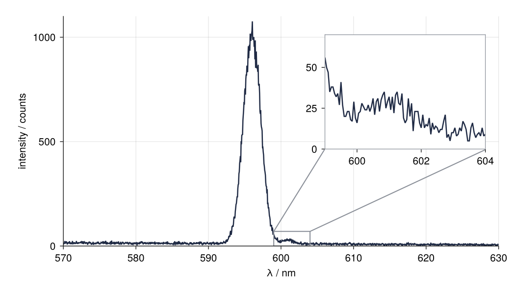
This is where we end up. Makie has no single call for it, so the figure is built from four pieces, one per step: a second Axis in the main axis's layout cell, translate! to draw it on top, the box and the lines drawn by hand, and tick labels measured at print size. You need what CairoMakie from the ground up covers: Figure, Axis, the grid of cells, with_theme, and sizes in points. Nothing about insets.

Setup

Install the two packages once with import Pkg; Pkg.add(["CairoMakie", "Distributions"]); Random and Printf ship with Julia. Distributions.jl is here only for the Poisson noise of photon counting. SITE is the look of every figure on this site, and PRINT the print size, 504 by 288 units, which are points when the figure is saved with pt_per_unit = 1 (Step 4 of the prerequisite). The four tuples at the end fix the limits, the zoom region, and the inset's place, and every step below reads them from there.

using CairoMakie, Random, Distributions, Printf

const INK, ACCENT, SECOND, MUTED = "#1f2a44", "#c8553d", "#2a7f9e", "#8a8f98"
SITE = Theme(
    size = (770, 396), fontsize = 17,
    palette = (color = [INK, ACCENT, SECOND, MUTED],),
    Axis = (topspinevisible = false, rightspinevisible = false, xgridvisible = true, ygridvisible = true),
    Lines = (linewidth = 2.5,),
)
set_theme!(SITE)
PRINT = Theme(
    size = (504, 288), fontsize = 10,                        # 7 x 4 in, in points
    Axis = (spinewidth = 0.6, xtickwidth = 0.6, ytickwidth = 0.6, xticksize = 3, yticksize = 3,
            xgridwidth = 0.5, ygridwidth = 0.5),
    Lines = (linewidth = 1.2,),
)

# ---- data: replace lam and counts with your own
line(lam, height, center, width) = height * exp(-0.5 * ((lam - center) / width)^2)
rng = Xoshiro(58)
lam = range(570, 630, length = 1201)                         # wavelength / nm, 0.05 nm steps
expected = @. 15 - 0.15 * (lam - 570) + line(lam, 1000, 596, 1.2) + line(lam, 20, 601, 0.7)
counts = [rand(rng, Poisson(e)) for e in expected]           # photon counting gives Poisson noise

xlim, ylim = (570, 630), (0, 1100)                           # main axis: nm, counts
region = (599, 604, 0, 70)                                   # zoom region: x0, x1 in nm, y0, y1 in counts
bounds = (0.60, 0.42, 0.37, 0.50)                            # inset: x0, y0, width, height, fractions of the main axis

mkpath("assets")
i = argmax(counts)
@printf("%d points from %.0f to %.0f nm, largest reading %d counts at %.2f nm\n",
        length(lam), first(lam), last(lam), counts[i], lam[i])

1201 points from 570 to 630 nm, largest reading 1076 counts at 596.05 nm

Step 1: Draw the spectrum at print size

The main figure is built the prerequisite's way, inside with_theme with Figure() as its first line, so that the figure takes the print theme. limits!(ax, x0, x1, y0, y1) sets both ranges in one call, xlims! and ylims! at once.

Copy

fig, ax = with_theme(merge(PRINT, SITE)) do
    fig = Figure()
    ax = Axis(fig[1, 1]; xlabel = "λ / nm", ylabel = "intensity / counts")
    lines!(ax, lam, counts; color = INK)
    limits!(ax, xlim..., ylim...)
    fig, ax
end

axis_h = ax.scene.viewport[].widths[2]                       # height of the plotting area / pt
@printf("main axis %.0f pt tall: 20 counts stand %.1f mm on paper\n",
        axis_h, 20 / (ylim[2] - ylim[1]) * axis_h * 25.4 / 72)
fig

main axis 225 pt tall: 20 counts stand 1.4 mm on paper

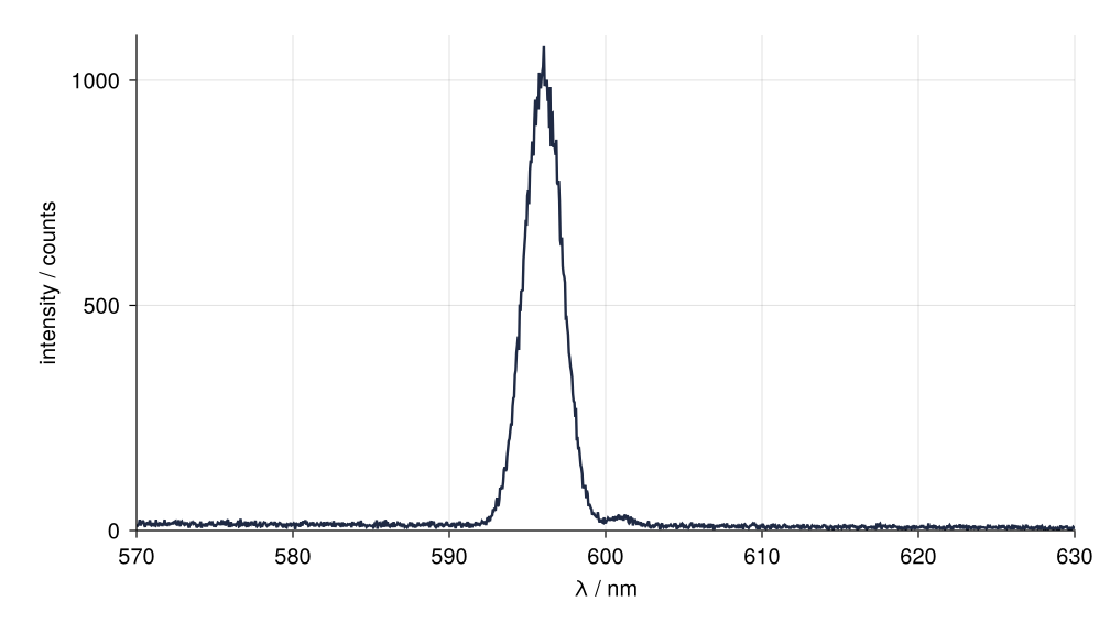
The satellite is a bump at the foot of the strong line, hardly thicker than the trace. The limits are set by hand rather than left to Makie because Step 4 turns fractions of the axis into nanometers and counts and needs the axis to run from exactly 570 to 630 nm; Pitfall 1 shows what happens otherwise. Every later step adds to this fig. Blocks added after the with_theme block has closed still follow the print theme, because they take it from the figure.

Step 2: Put a second Axis into the main axis's cell

A cell of the layout can hold more than one block. Calling Axis(fig[1, 1]) a second time puts a new axis into the cell ax already occupies, and four keywords size and place it. Relative(0.37) is a width as a share of the cell. The cell is the main axis's plotting area, the rectangle inside its spines with the tick labels outside it, so bounds reads as fractions of the main axis: lower-left corner at 0.60 and 0.42, size 0.37 by 0.50. A number for halign places the block in the room the cell has left over beside it, 0 flush left and 1 flush right. That room is 1 − 0.37 = 0.63 of the cell, so a left edge at 0.60 needs halign = 0.60 / 0.63; valign does the same upward.

Copy

x0, y0, w, h = bounds
inset = Axis(fig[1, 1]; width = Relative(w), height = Relative(h),
             halign = x0 / (1 - w), valign = y0 / (1 - h),
             backgroundcolor = :white, xgridvisible = false, ygridvisible = false)
lines!(inset, lam, counts; color = INK)
limits!(inset, region...)

outer, inner = ax.scene.viewport[], inset.scene.viewport[]
@printf("halign %.3f, valign %.3f; inset %.0f x %.0f pt\n", x0 / (1 - w), y0 / (1 - h), inner.widths...)
@printf("inset in fractions of the main axis: x0 %.3f, y0 %.3f, width %.3f, height %.3f\n",
        ((inner.origin .- outer.origin) ./ outer.widths)..., (inner.widths ./ outer.widths)...)
fig

halign 0.952, valign 0.840; inset 157 x 112 pt
inset in fractions of the main axis: x0 0.601, y0 0.422, width 0.369, height 0.498

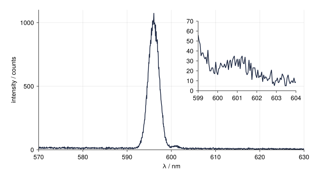
The viewport of an axis is the rectangle it occupies in the figure, and the fractions read back from the two viewports match bounds to within 0.002. The difference is the layout rounding positions and sizes to whole points. The inset is a full Axis with its own limits and shows only what is drawn into it, hence the second lines!. Its grid is off, since at 157 by 112 pt a grid only crowds the trace.

The placement is right; the drawing order is not. Four grid lines of the main axis run straight through the inset's white face, and the default ticks crowd it with six labels on x and eight on y.

Step 3: Draw the inset on top with translate!

CairoMakie does not draw a figure axis by axis. It collects every piece of it, from backgrounds to tick labels, sorts the pieces by their z value, the depth coordinate a 2D figure otherwise has no use for, and paints the lowest first. Every Axis puts its background at z = −100, its grid at −10, the data at 0, and its spines and ticks up to 20. So the main axis's grid is painted after the inset's white background, whatever order you created the two axes in. translate! shifts a scene, Makie's container for a group of drawn pieces, and inset.blockscene is the scene that holds all of the inset: face, frame, ticks, labels, and the plots inside. The scene field the prerequisite used (ax.scene) holds only the plots, so shifting inset.scene would leave the white face under the grid.

After the shift, the cell reads the z values back. Makie.collect_atomic_plots lists the atomic plots of a scene, the plain lines, polygons, and texts every drawn element breaks down into, and Makie.zvalue2d gives the z of each one that is visible. Both are unexported Makie internals: pin the Makie version in your project and expect to fix such calls after an upgrade.

Copy

zrange(block) = extrema(Makie.zvalue2d(p) for p in Makie.collect_atomic_plots(block.blockscene) if p.visible[])
translate!(inset.blockscene, 0, 0, 150)
@printf("z of the main axis from %.0f to %.0f, of the inset from %.0f to %.0f\n", zrange(ax)..., zrange(inset)...)
fig

z of the main axis from -100 to 20, of the inset from 50 to 170

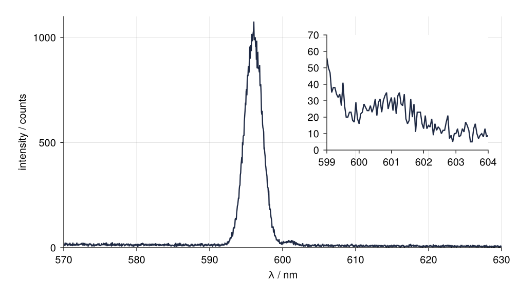
Shifted by 150, the inset's background lies above the highest piece of the main axis, and the grid lines are gone from its face: the verticals at 610 and 620 nm now stop at its frame. Any shift above 120 would do here, since the background at −100 has to clear the main axis's 20. With two insets that overlap, the one that belongs in front gets the larger shift. The inset now hides whatever lies under it, so Step 4 counts what that is.

Step 4: Mark the region with a box and two lines, and check what the inset covers

Makie draws neither the box nor the connecting lines, so both are lines! into the main axis, in its data units. The box is the five corners of region, closing on the first. The lines run from the box's upper-left and upper-right corners to the inset's lower-left and lower-right corners, so that neither crosses the box or the trace on the strong line's flank. With the default ticks they still cut through two of the inset's x labels; Step 5 deals with those. The inset's corners are known in fractions of the main axis, and on a linear axis with fixed limits a fraction f is xlim[1] + f * (xlim[2] - xlim[1]) in nm, and the same for counts: two one-line helpers. Box and lines are MUTED at a width of 1, as guides are on this site. The inset's frame turns the same gray and gets back the top and right spines the site theme hides.

Copy

to_x(f) = xlim[1] + f * (xlim[2] - xlim[1])                 # fraction of the main axis -> nm
to_y(f) = ylim[1] + f * (ylim[2] - ylim[1])                 # fraction of the main axis -> counts

xa, xb, ya, yb = region
guide = (color = MUTED, linewidth = 1)
lines!(ax, [xa, xb, xb, xa, xa], [ya, ya, yb, yb, ya]; guide...)
lines!(ax, [xa, to_x(x0)], [yb, to_y(y0)]; guide...)         # box upper-left to inset lower-left
lines!(ax, [xb, to_x(x0 + w)], [yb, to_y(y0)]; guide...)     # box upper-right to inset lower-right
inset.topspinevisible = inset.rightspinevisible = true
inset.leftspinecolor = inset.rightspinecolor = inset.bottomspinecolor = inset.topspinecolor = MUTED

points_under(x0, y0, w, h) = count(@. (to_x(x0) <= lam <= to_x(x0 + w)) & (to_y(y0) <= counts <= to_y(y0 + h)))
@printf("data points under the inset: %d\n", points_under(bounds...))
@printf("magnification: λ %.1f times, counts %.1f times\n",
        w * (xlim[2] - xlim[1]) / (xb - xa), h * (ylim[2] - ylim[1]) / (yb - ya))
fig

data points under the inset: 0
magnification: λ 4.4 times, counts 7.9 times

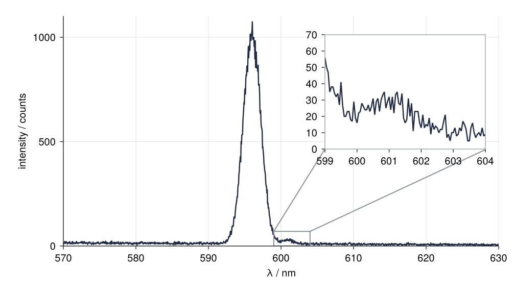
No data point lies under the inset. Since Step 3 made it opaque, only this count would tell you if one did (Pitfall 2).

The magnification is the inset's share of the main axis times the ratio of the ranges. The inset spans 0.37 × 60 = 22 nm of the main axis's width and shows 5 nm in it, so every nanometer is drawn 4.4 times as wide; the counts work the same way, 7.9 times. Drawn in the inset, the 20-count satellite takes up the height that about 160 counts take in the main axis. Nobody can judge its size by eye there, only from the inset's tick labels. So the labels stay, and Step 5 makes them legible.

Step 5: Keep the inset's tick labels readable at print size

Crowded tick labels get fewer ticks, not smaller labels: LinearTicks(3) asks for about three. Whether the labels then fit is a measurement, and it needs three things the prerequisite never showed.

An Axis holds two axis objects, inset.xaxis and inset.yaxis, each drawing the ticks, tick labels, and spine of its direction. Their field elements is a dictionary of those drawn parts by name, :ticklabels among them, and Makie.string_boundingboxes returns one box per label in figure units, which are points with PRINT. Both are internals again, with the same rule as in Step 3.

The boxes describe the text as laid out, and the layout is complete once the figure has been drawn. colorbuffer(fig) draws it into an image in memory, as save does, without writing a file. Measure after a draw, and draw again after anything that moves labels, such as new ticks or a new size.

The gap is edge to edge, the white space between neighboring boxes, not the distance between their centers.

Copy

mm(pt) = pt * 25.4 / 72                                      # 1 pt = 0.353 mm
function label_gaps(side, d)                                 # side: inset.xaxis or inset.yaxis; d = 1 across, 2 up
    boxes = sort(Makie.string_boundingboxes(side.elements[:ticklabels]); by = b -> minimum(b)[d])
    gaps = [minimum(b)[d] - maximum(a)[d] for (a, b) in zip(boxes, boxes[2:end])]
    return length(boxes), mm(minimum(gaps))
end
report(ticks) = @printf("%-15s %d labels on x, %4.1f mm apart; %d on y, %4.1f mm apart\n",
                        ticks, label_gaps(inset.xaxis, 1)..., label_gaps(inset.yaxis, 2)...)

colorbuffer(fig)                                             # draw, so that the labels are laid out
report("default ticks:")
inset.xticks = LinearTicks(3)
inset.yticks = LinearTicks(3)
colorbuffer(fig)                                             # the labels moved: draw again
report("LinearTicks(3):")
fig

default ticks:  6 labels on x,  5.2 mm apart; 8 on y,  1.5 mm apart
LinearTicks(3): 3 labels on x, 16.3 mm apart; 3 on y, 10.0 mm apart

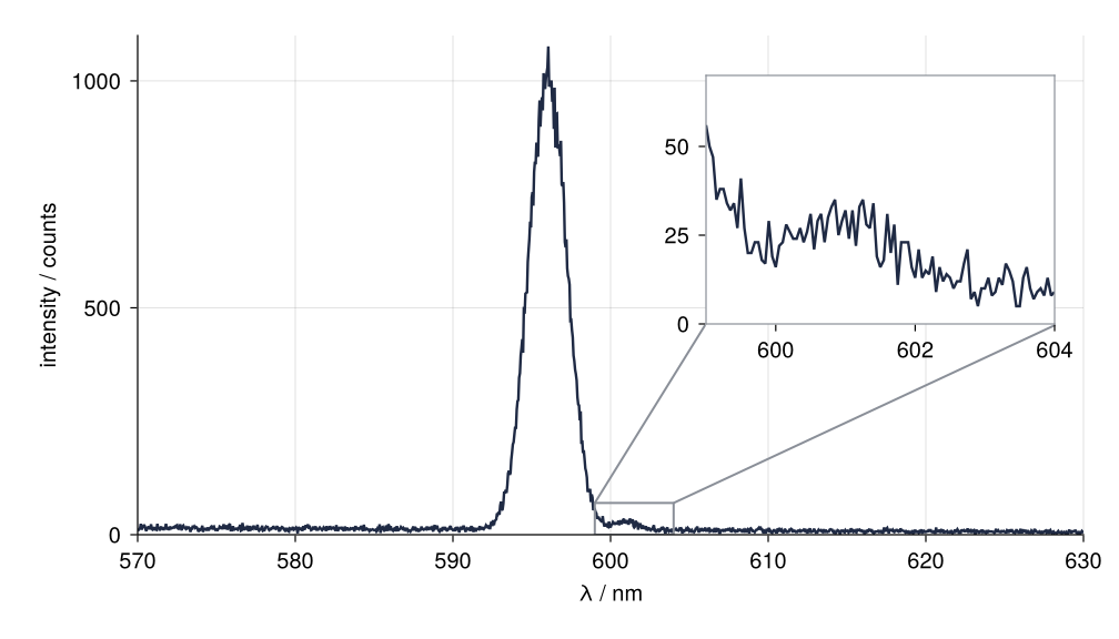
Two labels read as separate numbers when at least one digit's width of white lies between them, about 2 mm at 10 pt. The default labels on y miss it at 1.5 mm, and the connecting lines of Step 4 cut through the default 599 and 603 on x; three labels per axis leave 16 mm on x and 10 mm on y. A measurement holds only at the size it was taken at, which is why PRINT makes the figure at its printed size. For the paper, save("spectrum-inset.pdf", fig; pt_per_unit = 1) writes it out (Step 6 of the prerequisite).

Pitfalls

Lines that miss the inset's corners. Leave out limits!(ax, ...) and Makie pads the data range by 5 % on each side (xautolimitmargin and yautolimitmargin, 0.05 by default):

loose = Figure()
a = Axis(loose[1, 1])
lines!(a, lam, counts)
colorbuffer(loose)                                           # autolimits are final after a draw
lims = a.finallimits[]
@printf("without limits!: λ from %.0f to %.0f nm\n", minimum(lims)[1], maximum(lims)[1])

without limits!: λ from 567 to 633 nm

The fraction conversion of Step 4 still assumes 570 to 630 nm, so the connecting lines end beside the inset's corners while the box still sits right. Set the main limits by hand before computing the lines. On a log axis the conversion goes through the logarithm (Variations).

An inset that hides data. Move the inset left to x0 = 0.30 and it covers the top of the strong line without a warning, because Step 3 made it opaque and put it on top:

@printf("data points under the inset at x0 = 0.30: %d\n", points_under(0.30, y0, w, h))

data points under the inset at x0 = 0.30: 57

That is 57 readings of the line gone behind a white face. Choose the emptiest corner of the plot for the inset and rerun Step 4's count after every move; it must read 0. When every corner holds data, make room above them with a larger ylim[2].

Tick labels lost at print size. Crowded inset ticks tempt you to set xticklabelsize = 6. That makes them the smallest text in the paper, and the journal may shrink them further: a figure 7 in (17.8 cm) wide placed in an 8.6 cm column is scaled to 0.48, and the 6 pt labels come out at 2.9 pt. Keep the labels at the size of the main ticks, thin them with LinearTicks(3), make the figure at its final width in the first place, and repeat the label_gaps measurement. Removing the labels does not help either, for the reason in Step 4.

Variations

• One journal column. Set size = (245, 158) in PRINT, 8.6 cm wide; bounds keeps its meaning. Draw again with colorbuffer, then rerun label_gaps.
• Two insets. A third Axis(fig[1, 1]; ...) with its own bounds, region, box, and lines; if it overlaps the first, give it the larger shift, by Step 3's rule (say 200).
• A logarithmic main axis. With yscale = log10 and limits ylo to yhi, a fraction f is 10^(log10(ylo) + f * (log10(yhi) - log10(ylo))) counts. bounds and Relative stay as they are, because they live in the layout, not in the data.
• A fit in the inset. The inset is a full Axis, so a model and its band go in with the same calls as in Fit a curve with error bars and draw a confidence band in Julia.

Cheat sheet

limits!(ax, x0, x1, y0, y1)                                  # fixed limits: fractions convert exactly
inset = Axis(fig[1, 1]; width = Relative(w), height = Relative(h),   # same cell as ax
             halign = fx / (1 - w), valign = fy / (1 - h))  # lower-left corner at (fx, fy) of ax
lines!(inset, x, y); limits!(inset, rx0, rx1, ry0, ry1)       # the zoom region
translate!(inset.blockscene, 0, 0, 150)                      # draw the inset over the main axis
to_x(f) = x0 + f * (x1 - x0); to_y(f) = y0 + f * (y1 - y0)  # fraction of ax -> data, linear axes
lines!(ax, [rx0, to_x(fx)], [ry1, to_y(fy)]; color = MUTED, linewidth = 1)       # one connecting line
inset.xticks = LinearTicks(3)                                # fewer ticks, not smaller labels
save("fig.pdf", fig; pt_per_unit = 1)                        # a unit is a point

Further reading

• The Makie documentation: the Axis reference for width, height, halign, valign, and xticks, and the Layout tutorial for cells and blocks.
• Simon Danisch and Julius Krumbiegel, "Makie.jl: Flexible high-performance data visualization for Julia", Journal of Open Source Software 6 (2021) 3349.
• Related tutorials on this site: CairoMakie from the ground up: a two-panel figure for one journal column, for the print theme and saving; Zoom into a detail of a Matplotlib plot with an inset, the same figure in Python, where two calls do the work; Fit a curve with error bars and draw a confidence band in Julia.
• Download the notebook. It was executed with the library versions in the header.