Classification with MLJ.jl: telling two populations apart

The problem: which population did this event come from?

Take 2,000 events, 600 of them signal and 1,400 background, each carrying two measured numbers, x₁ and x₂, with the two populations overlapping. Your own two classes fit the same mold: tumor cells against healthy ones, quartz against feldspar under the microscope, a particle track against detector noise. You want a rule that names the population of a new event from its two numbers, and an honest estimate of how often it names it correctly. Such a rule is a classifier, and its fraction of correct answers is its accuracy. MLJ.jl is Julia's machine-learning toolbox for the job: one interface in front of models that live in many separate packages.

Two numbers bracket every classifier before anything is fitted. Answering "background" for every event scores 70.0 % and needs no measurement at all. The best possible rule, one that knows both populations exactly, scores 82.5 %, and nothing beats it, because an event inside the overlap could have come from either side. Real data never tell you that second number. These data can, because they are drawn from two Gaussians written down in Setup.

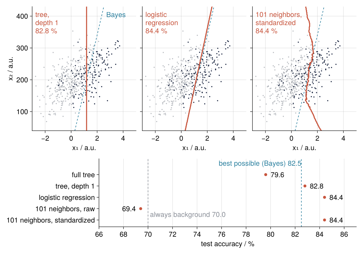
Top: 500 test events, x₂ against x₁ in a.u., signal dark and background gray. Red: the boundaries of a depth-1 tree (vertical), logistic regression (slanted), and 101 standardized neighbors (bent), each beside the dashed Bayes boundary. Bottom: five test accuracies between the 70.0 % floor and the 82.5 % ceiling.

That is the destination. A decision boundary is the line where a classifier switches its answer from background to signal. Each top panel draws one across the test events, beside the dashed boundary of the best possible rule, Bayes' rule, and the bottom panel lists how five rules score on those events. The three tuned ones reach 82.8 % to 84.4 %, above the 82.5 % because these 500 events are an easy draw, as Step 6 shows. A tree on its default settings stops at 79.6 %, and the neighbors without standardization at 69.4 %, under the floor. Six steps build the figure.

Setup

Install the packages once with import Pkg; Pkg.add(["MLJ", "MLJDecisionTreeInterface", "DecisionTree", "MLJLinearModels", "NearestNeighborModels", "Distributions", "CairoMakie"]); Random and Printf ship with Julia. MLJ itself holds no models. Each lives in its own package, and @load DecisionTreeClassifier pkg=DecisionTree loads that package's MLJ interface and returns the model's type, bound below to the short name Tree; like using, it is needed once per session. A fresh session runs the notebook in about two and a half minutes, nearly all of it compilation: the same fits repeated in the pitfalls take a second or two.

MLJ takes the features X as a table, here a NamedTuple of columns (a table from DataFrames.jl works too), and the labels y as a categorical vector. It checks each column's scientific type, or scitype: a classifier wants Continuous features and OrderedFactor or Multiclass labels. Integer columns and labels coded 0 and 1 arrive as Count, which a classifier refuses; coerce(X, Count => Continuous) and coerce(y, OrderedFactor) convert them, and next to Distributions, as here, the first needs MLJ.Continuous. The figure cells use CairoMakie; nothing in the text depends on reading them.

using MLJ, Distributions, Random, Printf, CairoMakie
import DecisionTree          # for the depth and leaf count of a fitted tree

Tree = @load DecisionTreeClassifier pkg=DecisionTree verbosity=0
LogisticClassifier = @load LogisticClassifier pkg=MLJLinearModels verbosity=0
KNNClassifier = @load KNNClassifier pkg=NearestNeighborModels verbosity=0

const INK, ACCENT, SECOND, MUTED = "#1f2a44", "#c8553d", "#2a7f9e", "#8a8f98"
set_theme!(Theme(
    size = (770, 396), fontsize = 17,
    palette = (color = [INK, ACCENT, SECOND, MUTED],),
    Axis = (topspinevisible = false, rightspinevisible = false, xgridvisible = true, ygridvisible = true),
    Lines = (linewidth = 2.5,),
))

mu_signal = [1.6, 220.0]
mu_background = [0.0, 200.0]
Σ = [1.0 25.0;        # x1 has sd 1, x2 has sd 50,
     25.0 2500.0]     # and their correlation is 25 / (1 * 50) = 0.5
P_signal, P_background = MvNormal(mu_signal, Σ), MvNormal(mu_background, Σ)

rng = Xoshiro(40)
S, B = rand(rng, P_signal, 600), rand(rng, P_background, 1400)   # 2 × n, one column per event
X = (x1 = [S[1, :]; B[1, :]], x2 = [S[2, :]; B[2, :]])
y = coerce([fill("signal", 600); fill("background", 1400)], OrderedFactor)

println("scitype of X: ", scitype(X))
println("scitype of y: ", scitype(y))
@printf("levels %s, signal fraction %.3f\n", join(levels(y), " < "), mean(y .== "signal"))

scitype of X: Table{AbstractVector{ScientificTypesBase.Continuous}}
scitype of y: AbstractVector{OrderedFactor{2}}
levels background < signal, signal fraction 0.300

Continuous columns and two ordered levels, as a classifier needs, with three events in ten signal.

Step 1: Split the data into a training and a test set

Score a rule on its own training material and it flatters itself, by 20 points in Step 2. A quarter of the events therefore form a test set, kept out of sight until the end and used once. Every model learns from the remaining three quarters, the training set. MLJ splits row numbers, not the data:

train, test = partition(eachindex(y), 0.75; shuffle = true, stratify = y, rng = 0)
signal_fraction(rows) = mean(y[rows] .== "signal")
@printf("training %4d events, signal fraction %.3f\n", length(train), signal_fraction(train))
@printf("test     %4d events, signal fraction %.3f\n", length(test), signal_fraction(test))

training 1500 events, signal fraction 0.300
test      500 events, signal fraction 0.300

stratify = y keeps the signal fraction at 0.300 on both sides. shuffle = true matters because Setup put all the signal first, and rng = 0 fixes the shuffle. From here on every call that fits or predicts takes rows = train or rows = test, and X and y are never copied. The training set:

is_signal = y[train] .== "signal"
fig = Figure()
ax = Axis(fig[1, 1], xlabel = "x₁ / a.u.", ylabel = "x₂ / a.u.")
scatter!(ax, X.x1[train][.!is_signal], X.x2[train][.!is_signal], color = (MUTED, 0.6), markersize = 5)
scatter!(ax, X.x1[train][is_signal], X.x2[train][is_signal], color = INK, markersize = 5)
text!(ax, -3.0, 330, text = "background", color = MUTED)
text!(ax, 3.4, 110, text = "signal", color = INK)
fig

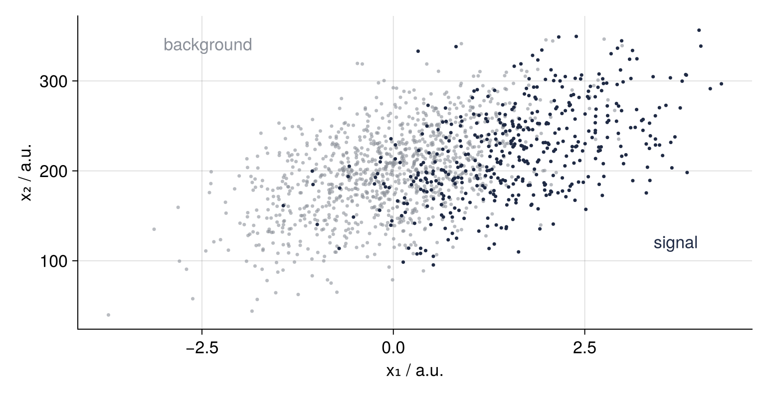
The 1,500 training events, x₂ against x₁ in a.u. Dark dots: signal, gray dots: background. The clouds overlap, and x₂ covers roughly 40 times the range of x₁.

Where the clouds overlap, every rule makes mistakes. Read the tick labels too: x₂ covers roughly 40 times the range of x₁, and Steps 4 and 5 pay for that.

Step 2: Fit a decision tree and score it

A decision tree sorts events with yes-or-no questions, each about a single feature ("x₁ < 1.2?"). Every answer leads to a further question, and the splitting goes on until every region, called a leaf, holds mostly one class. A new event walks down to its leaf and takes the leaf's majority label. The builder breaks ties between equally good questions at random, hence the seed.

MLJ keeps the model apart from the data. The model, Tree(rng = 0) with the type Setup loaded, holds nothing but its settings. machine binds it to the data, and fit! learns from the rows you name. predict returns, for every event, a probability for each class, and predict_mode picks the most likely class, which is the label:

tree = Tree(rng = 0)
mach = machine(tree, X, y)
fit!(mach, rows = train, verbosity = 0)
println("predicted: ", join(predict_mode(mach, rows = test[1:8]), "  "))
println("true:      ", join(y[test[1:8]], "  "))

predicted: signal  signal  signal  signal  signal  background  background  background
true:      signal  signal  signal  signal  signal  signal  signal  signal

On the first eight test events, all signal, the tree is wrong three times. accuracy compares predicted with true labels, and the helper accuracy_on wraps the two calls. fitted_params returns what fitting learned, here the tree itself. DecisionTree's depth and length, the leaf count, measure the tree:

accuracy_on(mach, rows) = accuracy(predict_mode(mach, rows = rows), y[rows])
@printf("accuracy on training %.3f, on test %.3f\n", accuracy_on(mach, train), accuracy_on(mach, test))
raw_tree = fitted_params(mach).raw_tree
@printf("depth %d, leaves %d\n", DecisionTree.depth(raw_tree), DecisionTree.length(raw_tree))

accuracy on training 1.000, on test 0.796
depth 26, leaves 253

A perfect training score and 79.6 % on the test set. With 26 levels and 253 leaves, about six training events per leaf, the tree has memorized these particular events instead of the two populations behind them. That is overfitting, and the 79.6 % is what counts, 9.6 points above always answering background.

The settings a model takes before it sees any data are its hyperparameters. For a tree the one that matters most is max_depth, how many questions an event may face on its way down, unlimited by default.

Step 3: Choose the tree depth with cross-validation

Choosing max_depth by its test score is tempting and wrong: the test set would share in the choice, and its score would flatter the model. Cross-validation answers the question without the test set. The training set is dealt into five parts, called folds; a model is fitted on four and scored on the fifth, until every fold has been scored once. StratifiedCV keeps the class ratio in every fold (CV is the plain version). evaluate takes a model and the data, builds one machine, and refits it from scratch on each fold:

folds() = StratifiedCV(nfolds = 5, shuffle = true, rng = 0)
depths = 1:10
cv_mean, cv_sd, train_acc = Float64[], Float64[], Float64[]
for d in depths
    e = evaluate(Tree(max_depth = d, rng = 0), X, y; rows = train,
                 resampling = folds(), measure = accuracy, verbosity = 0)
    push!(cv_mean, e.measurement[1])
    push!(cv_sd, std(e.per_fold[1]))
    m = fit!(machine(Tree(max_depth = d, rng = 0), X, y), rows = train, verbosity = 0)
    push!(train_acc, accuracy_on(m, train))
    @printf("max_depth %2d   CV %.3f ± %.3f   training %.3f\n", d, cv_mean[end], cv_sd[end], train_acc[end])
end

max_depth  1   CV 0.838 ± 0.022   training 0.839
max_depth  2   CV 0.838 ± 0.022   training 0.839
max_depth  3   CV 0.835 ± 0.020   training 0.839
max_depth  4   CV 0.839 ± 0.018   training 0.856
max_depth  5   CV 0.837 ± 0.023   training 0.862
max_depth  6   CV 0.825 ± 0.032   training 0.877
max_depth  7   CV 0.824 ± 0.026   training 0.884
max_depth  8   CV 0.820 ± 0.022   training 0.898
max_depth  9   CV 0.812 ± 0.027   training 0.907
max_depth 10   CV 0.803 ± 0.025   training 0.917

folds() builds a fresh StratifiedCV for every call: one shared object draws from the same generator at every use and would cut different folds for every depth. measure may be a list, so measurement and per_fold hold one entry per measure; [1] takes the only one.

Training accuracy climbs from 83.9 % to 91.7 %, while the cross-validated accuracy stays near 83.8 % to depth 5 and, with each further level fitting noise, slides to 80.3 % at depth 10:

fig = Figure()
ax = Axis(fig[1, 1], xlabel = "max_depth", ylabel = "accuracy / %", xticks = depths)
band!(ax, depths, 100 .* (cv_mean .- cv_sd), 100 .* (cv_mean .+ cv_sd), color = (ACCENT, 0.30))
lines!(ax, depths, 100 .* train_acc, color = MUTED)
scatterlines!(ax, depths, 100 .* cv_mean, color = ACCENT, markersize = 10)
hlines!(ax, 70, color = MUTED, linestyle = :dash, linewidth = 1.4)
text!(ax, 6.2, 88.5, text = "training set", color = MUTED, align = (:right, :bottom))
text!(ax, 10, 77, text = "cross-validated (± fold sd)", color = ACCENT, align = (:right, :top))
text!(ax, 10, 69.6, text = "always background", color = MUTED, align = (:right, :top))
lines!(ax, [1, 1.6], [100 * cv_mean[1], 75.5], color = ACCENT, linewidth = 1.4)
text!(ax, 1.6, 75.5, text = @sprintf("depth 1: %.1f %%", 100 * cv_mean[1]), color = ACCENT, align = (:left, :top))
ylims!(ax, 66, 94)
fig

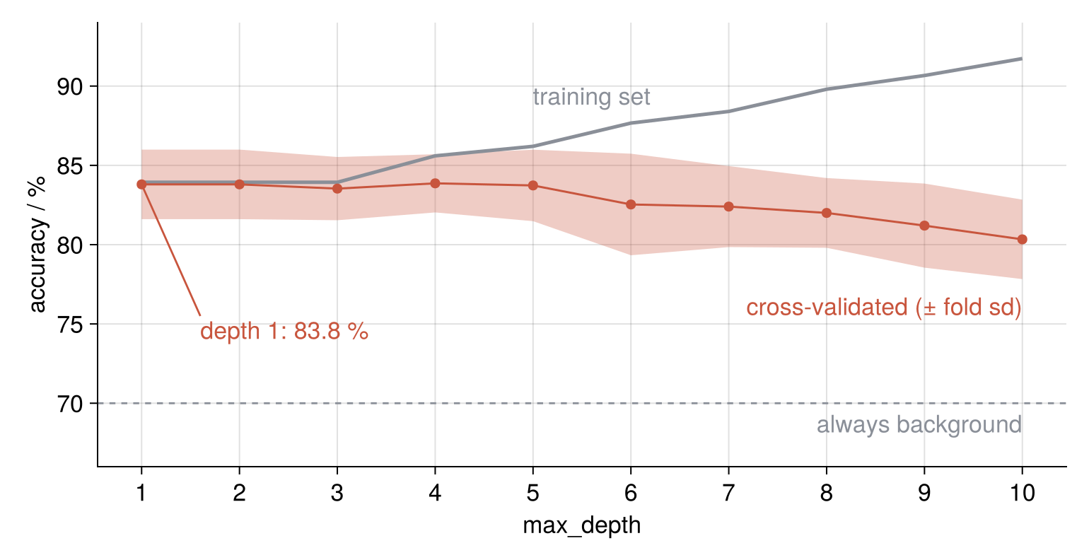
Decision tree accuracy in % against max_depth from 1 to 10. Red dots and band: cross-validated mean and fold spread, flat near 84 % up to depth 5, then falling; depth 1 chosen, within one fold sd of the best. Gray line: training accuracy, climbing past 91 %. Dashed: always background at 70 %.

With a fold spread of about 2 points the decimals are noise, and choosing needs a rule. Take the best cross-validated mean, here 83.9 % at depth 4. A simpler setting whose mean lies within the best one's fold sd, 1.8 points, is a tie with it, and among ties take the simplest, which has the least room to fit noise. For a tree, simpler means shallower, and depth 1 at 83.8 % is inside the margin: the rule chooses a single question.

Refit that tree on all 1,500 training events and give it its one look at the test set:

tree1 = fit!(machine(Tree(max_depth = 1, rng = 0), X, y), rows = train, verbosity = 0)
@printf("depth 1: test accuracy %.3f\n", accuracy_on(tree1, test))
fitted_params(tree1).tree

depth 1: test accuracy 0.828

x1 < 1.195
├─ background (956/1103)
└─ signal (303/397)

The one question is x₁ < 1.195, and it scores 82.8 %, 3.2 points better than the tree with 253 leaves.

Step 4: Fit a logistic regression

Logistic regression adds up the features with weights, plus a constant, to a number z, and the logistic function \(1/(1 + e^{-z})\) turns z into a probability of signal between 0 and 1. Signal is called where that probability passes 0.5, which is where z passes zero, so the decision boundary is the straight line z = 0. Same calls, new model:

logreg = fit!(machine(LogisticClassifier(), X, y), rows = train, verbosity = 0)
@printf("test accuracy %.3f\n", accuracy_on(logreg, test))
ŷ = predict(logreg, rows = test[1:3])
println("P(background) of three test events: ", round.(pdf.(ŷ, "background"), digits = 3))
println("P(signal) of the same events:       ", round.(pdf.(ŷ, "signal"), digits = 3))
w = fitted_params(logreg).coefs
@printf("weights: x1 %.3f, x2 %.4f\n", last(w[1]), last(w[2]))

test accuracy 0.844
P(background) of three test events: [0.266, 0.232, 0.67]
P(signal) of the same events:       [0.734, 0.768, 0.33]
weights: x1 2.042, x2 -0.0108

84.4 %, untuned. When two Gaussian populations share one covariance matrix, the best possible rule draws a straight line too, and a straight line is all this method can draw. On a prediction, pdf gives the probability of a class, not a density. coefs holds the weights as pairs of feature name and weight.

The weight of x₂ is 189 times smaller than that of x₁, and that reflects the unit of x₂, not how much x₂ matters. Measure x₂ in a unit 50 times coarser and its weight grows by the same factor while the line stays put: the best line does not depend on units. Finding it does. LogisticClassifier finds its weights with an optimizer, a search that adjusts them step by step until the fit stops improving, and weights 189 times apart make that search hard. Refit it on 20 other seeded splits:

function split_scores(model)        # test accuracy on the splits with seeds 1 to 20
    map(1:20) do seed
        tr, te = partition(eachindex(y), 0.75; shuffle = true, stratify = y, rng = seed)
        accuracy_on(fit!(machine(model, X, y), rows = tr, verbosity = 0), te)
    end
end
lr_raw = split_scores(LogisticClassifier())
at_floor = lr_raw .== 0.7
@printf("%d of 20 splits at the floor; the other %d from %.3f to %.3f\n",
        count(at_floor), count(.!at_floor), extrema(lr_raw[.!at_floor])...)

3 of 20 splits at the floor; the other 17 from 0.826 to 0.872

On 3 splits the search stopped with the weight of x₁ near zero and called every event background, without a warning, while the other 17 score 82.6 % to 87.2 %. A tree is blind to units, because rescaling x₂ rescales its thresholds with it. Logistic regression is not: put the standardizer of Step 5 in front of it whenever the features differ in scale.

Step 5: Put a standardizer in front of nearest neighbors with a pipeline

Nearest neighbors finds the K training events nearest to a new one and lets them vote on its label; K is the hyperparameter. Nearness is measured as the Euclidean distance \(\sqrt{\Delta x_1^2 + \Delta x_2^2}\), and that is where units bite: x₂ spreads over about 50 units, x₁ over about 1, so x₂ alone picks the neighbors. A Standardizer shifts each Continuous column by its mean and divides it by its sd, after which the features weigh the same. Any method built on distances needs one in front.

Standardizer() |> KNNClassifier(K = 51) joins the two into one model, a pipeline; between models, |> builds Pipeline(Standardizer(), KNNClassifier(K = 51)) and fits nothing. Inside evaluate the pipeline refits its standardizer on the four training folds of each round. Standardize the 1,500 events once beforehand instead, and the mean and sd that shape every round include the events of the fold being scored: the model has seen part of its exam. The raw classifier runs alongside:

println("    K   raw            standardized")
for K in [1, 5, 15, 25, 51, 101]
    raw = evaluate(KNNClassifier(K = K), X, y; rows = train,
                   resampling = folds(), measure = accuracy, verbosity = 0)
    scaled = evaluate(Standardizer() |> KNNClassifier(K = K), X, y; rows = train,
                    resampling = folds(), measure = accuracy, verbosity = 0)
    @printf("%5d   %.3f ± %.3f   %.3f ± %.3f\n", K, raw.measurement[1], std(raw.per_fold[1]),
            scaled.measurement[1], std(scaled.per_fold[1]))
end

    K   raw            standardized
    1   0.743 ± 0.021   0.765 ± 0.033
    5   0.775 ± 0.019   0.826 ± 0.022
   15   0.749 ± 0.015   0.831 ± 0.020
   25   0.735 ± 0.007   0.838 ± 0.027
   51   0.716 ± 0.022   0.844 ± 0.024
  101   0.701 ± 0.006   0.837 ± 0.022

Standardized, the accuracy rises from 76.5 % at K = 1 to 84.4 % at K = 51 and holds near 84 % at K = 101. Raw, it peaks at 77.5 % for K = 5 and sinks to the floor, 70.1 %, at K = 101: a hundred neighbors picked by x₂ are mostly background. For neighbors, simpler means more of them, which average over more events and draw a smoother boundary. Step 3's rule takes the best mean, 84.4 ± 2.4 % at K = 51, and then K = 101, the largest within the margin:

knn = fit!(machine(Standardizer() |> KNNClassifier(K = 101), X, y), rows = train, verbosity = 0)
@printf("K = 101: test accuracy %.3f\n", accuracy_on(knn, test))
st = fitted_params(knn).standardizer
@printf("standardizer mean: x1 %6.2f, x2 %6.2f\n", st.means...)
@printf("standardizer sd:   x1 %6.2f, x2 %6.2f\n", st.stds...)

K = 101: test accuracy 0.844
standardizer mean: x1   0.46, x2 206.53
standardizer sd:   x1   1.24, x2  50.65

84.4 %, level with logistic regression. A pipeline's fitted parameters are grouped by component, hence .standardizer. Its sds, 1.24 for x₁ and 50.65 for x₂, come from the training rows alone.

Step 6: Compare with the best possible rule

Because both Gaussians are known, the best rule has a formula, Bayes' rule. Weigh the signal density at the event's position by 0.3 and the background density by 0.7, and call the event signal if the first wins. The weights are the priors: the share of each class you expect before any measurement. The MvNormals of Setup apply it, in the collapsed cell, to a million fresh events and to the events at hand:

Show code

bayes(x) = 0.3 * pdf(P_signal, x) > 0.7 * pdf(P_background, x)    # x = [x1, x2]; true means signal

rng_fresh = Xoshiro(41)
n_signal = rand(rng_fresh, Binomial(10^6, 0.3))
fresh_signal = rand(rng_fresh, P_signal, n_signal)
fresh_background = rand(rng_fresh, P_background, 10^6 - n_signal)
acc_ceiling = (count(bayes, eachcol(fresh_signal)) + count(!bayes, eachcol(fresh_background))) / 10^6

test_events = [[X.x1[i], X.x2[i]] for i in test]
acc_bayes_test = mean(bayes.(test_events) .== (y[test] .== "signal"))
all_events = [[X.x1[i], X.x2[i]] for i in eachindex(y)]
acc_bayes_all = mean(bayes.(all_events) .== (y .== "signal"))
@printf("Bayes rule, 10^6 fresh events:   %.3f\n", acc_ceiling)
@printf("Bayes rule, all 2,000 events:    %.3f\n", acc_bayes_all)
@printf("Bayes rule, the 500 test events: %.3f\n", acc_bayes_test)

Bayes rule, 10^6 fresh events:   0.825
Bayes rule, all 2,000 events:    0.843
Bayes rule, the 500 test events: 0.848

The ceiling is 82.5 %, while the same rule gets 84.3 % of the 2,000 events right and 84.8 % of the test events: an easy sample. For the floor, ConstantClassifier ignores the features and predicts the training set's class frequencies, whose most likely class is background. The raw neighbors get the same K = 101 and are fitted only now, after every choice is made:

constant = fit!(machine(ConstantClassifier(), X, y), rows = train, verbosity = 0)
knn_raw = fit!(machine(KNNClassifier(K = 101), X, y), rows = train, verbosity = 0)
results = ["full tree" => mach, "tree, depth 1" => tree1, "logistic regression" => logreg,
           "101 neighbors, raw" => knn_raw, "101 neighbors, standardized" => knn]
acc_floor = accuracy_on(constant, test)
@printf("%-28s %.3f\n", "always background", acc_floor)
for (name, m) in results
    @printf("%-28s %.3f\n", name, accuracy_on(m, test))
end

always background            0.700
full tree                    0.796
tree, depth 1                0.828
logistic regression          0.844
101 neighbors, raw           0.694
101 neighbors, standardized  0.844

To draw a boundary, each machine predicts a label at every point of a 300 × 300 grid, and the boundary is where its answers flip; for Bayes' rule, it is where the two weighted densities are equal.

Show code

g1, g2 = range(-3, 5, length = 300), range(40, 430, length = 300)
grid = (x1 = repeat(g1, outer = 300), x2 = repeat(g2, inner = 300))    # point (i, j) at index i + 300(j - 1)
on_grid(v) = reshape(v, 300, 300)
signal_map(m) = on_grid(Float64.(predict_mode(m, grid) .== "signal"))
pts = [grid.x1'; grid.x2']
log_ratio = on_grid(log(0.3) .+ logpdf(P_signal, pts) .- log(0.7) .- logpdf(P_background, pts))

fig = Figure(size = (880, 616))
top = fig[1, 1] = GridLayout(alignmode = Outside())    # the panels take the full width, not the bottom axis's
is_signal = y[test] .== "signal"
panels = [("tree,\ndepth 1", tree1), ("logistic\nregression", logreg), ("101 neighbors,\nstandardized", knn)]
axs = [Axis(top[1, i], xlabel = "x₁ / a.u.", xticks = [-2, 0, 2, 4]) for i in 1:3]
linkaxes!(axs...)
for (i, (name, m)) in enumerate(panels)
    ax = axs[i]
    scatter!(ax, X.x1[test][.!is_signal], X.x2[test][.!is_signal], color = (MUTED, 0.6), markersize = 4)
    scatter!(ax, X.x1[test][is_signal], X.x2[test][is_signal], color = INK, markersize = 4)
    contour!(ax, g1, g2, log_ratio, levels = [0], color = SECOND, linewidth = 1.4, linestyle = :dash)
    contour!(ax, g1, g2, signal_map(m), levels = [0.5], color = ACCENT, linewidth = 2.5)
    text!(ax, 0.03, 0.97, text = @sprintf("%s\n%.1f %%", name, 100 * accuracy_on(m, test)),
          space = :relative, align = (:left, :top), color = ACCENT)
    i == 1 ? (ax.ylabel = "x₂ / a.u.") : (ax.yticklabelsvisible = false)
end
text!(axs[1], 2.7, 405, text = "Bayes", color = SECOND, align = (:left, :center))
limits!(axs[1], -3, 5, 40, 430)
colgap!(top, 10)

names = first.(results)
acc = [100 * accuracy_on(m, test) for m in last.(results)]
rows = reverse(0:length(names) - 1)
bottom = fig[2, 1] = GridLayout(alignmode = Outside())
ax = Axis(bottom[1, 1], xlabel = "test accuracy / %", xticks = 66:2:86, yticks = (rows, names), ygridvisible = false)
for (level, color, label, side, height) in
        [(100 * acc_ceiling, SECOND, @sprintf("best possible (Bayes) %.1f", 100 * acc_ceiling), :right, length(names) - 0.35),
         (100 * acc_floor, MUTED, @sprintf(" always background %.1f", 100 * acc_floor), :left, 0.5)]   # floor label between rows
    vlines!(ax, level, color = color, linestyle = :dash, linewidth = 1.4)
    text!(ax, level, height, text = label, color = color, align = (side, side == :left ? :center : :bottom))
end
scatter!(ax, acc, rows, color = ACCENT, markersize = 10)
for (a, r) in zip(acc, rows)
    left = a < 70.5        # keep the value clear of the floor line
    text!(ax, a + (left ? -0.4 : 0.4), r, text = @sprintf("%.1f", a), align = (left ? :right : :left, :center))
end
limits!(ax, 66, 87, -0.6, length(names) + 0.4)
rowsize!(fig.layout, 1, Relative(0.62))
fig

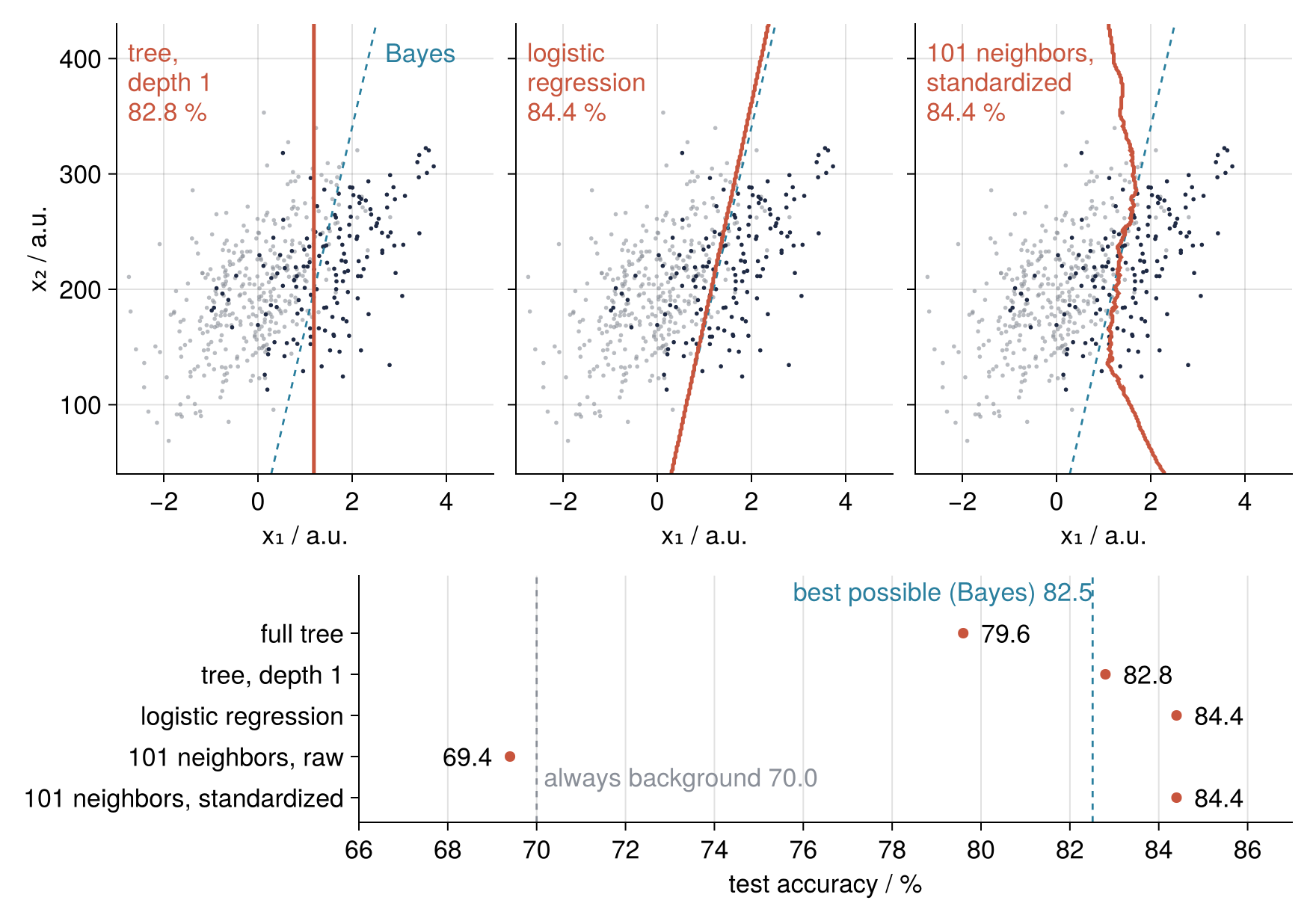
Top: 500 test events, x₂ against x₁ in a.u., signal dark and background gray. Red: decision boundaries of a depth-1 tree, logistic regression, and 101 standardized neighbors. Dashed blue: the Bayes boundary. Bottom: test accuracy of five classifiers in %, against the 70.0 floor and the 82.5 ceiling.

The tuned tree's boundary is a vertical line at x₁ = 1.195, the logistic line nearly covers the dashed Bayes line, and the standardized neighbors' line crosses it where events are dense and bends away above x₂ ≈ 330 and below 120, where few are left to vote. Any accuracy from 500 events carries a standard error, the scatter you would see between repeated samples of 500, of \(\sqrt{0.84 \cdot 0.16 / 500} \approx 1.6\) points (HypothesisTests.jl from the ground up treats such uncertainties). So 82.8 %, 84.4 %, and 84.8 % lie within 1.25 standard errors of each other, and no tuned rule can be told apart from the best one.

Pitfalls

Choosing on the test set. Here is what the test set says about max_depth if you ask it directly:

test_acc = [accuracy_on(fit!(machine(Tree(max_depth = d, rng = 0), X, y), rows = train, verbosity = 0), test)
            for d in depths]
println("test accuracy by depth: ", join([@sprintf("%.3f", a) for a in test_acc], " "))
println("best on the test set: depth ", depths[argmax(test_acc)])

test accuracy by depth: 0.828 0.828 0.828 0.834 0.828 0.820 0.812 0.810 0.814 0.814
best on the test set: depth 4

Depth 4 wins with 83.4 %, ahead of the depth 1 that cross-validation chose (82.8 %). The 0.6 points are well under one standard error, the kind of gap that ten looks at one test set turn up by chance, and the winner's score is optimistic by construction. A test set that has steered a decision has become training data, and standardizing all 2,000 events before the split leaks the same way, more quietly (Step 5). Make every choice by cross-validation on train, and touch test once, at the end.

An unseeded split. Change only the split and the reported accuracy changes with it. To see by how much, score the standardized logistic regression and the full tree on the 20 seeded splits of Step 4:

lr_std, full_tree = split_scores(Standardizer() |> LogisticClassifier()), split_scores(Tree(rng = 0))
for (name, a) in ["logistic, standardized" => lr_std, "full tree" => full_tree]
    @printf("%-23s %.3f to %.3f, %d of 20 at the floor\n", name, extrema(a)..., count(==(0.7), a))
end

logistic, standardized  0.824 to 0.876, 0 of 20 at the floor
full tree               0.748 to 0.794, 0 of 20 at the floor

The standardized logistic regression moves between 82.4 % and 87.6 %, its top 5 points above the ceiling, because all 20 test sets come from the same easy 2,000 events and each scatters by 1.6 points around them. Behind the standardizer it never ends at the floor. The full tree moves between 74.8 % and 79.4 %. partition draws its shuffle at random, and so does the tree builder, from Julia's global generator unless given rng. Pass rng to both, and report a cross-validated mean and its fold spread, not the third digit of one split.

An accuracy without its baseline. 69.4 % looks respectable next to nothing, and poor next to the 70.0 % of always answering background (the raw neighbors of Step 6). When one class dominates, guessing it already scores well above 50 %. Fit a ConstantClassifier beside every model, and when signal is the point, count it separately. confmat tabulates predicted against true classes:

confmat(predict_mode(knn_raw, rows = test), y[test])

           ┌─────────────────────┐
           │    Ground Truth     │
┌──────────┼──────────┬──────────┤
│Predicted │backgrou… │  signal  │
├──────────┼──────────┼──────────┤
│backgrou… │   338    │   141    │
├──────────┼──────────┼──────────┤
│  signal  │    12    │    9     │
└──────────┴──────────┴──────────┘

MLJ takes the prediction first and the truth second, and the display puts the prediction in rows and the truth, "Ground Truth", in columns. Read the labels rather than assume the orientation. The raw neighbors label 9 of the 150 signal events signal, 6 %.

Variations

TunedModel replaces the loops. TunedModel(model = Tree(rng = 0), range = range(Tree(), :max_depth, values = 1:10), tuning = Grid(), resampling = StratifiedCV(nfolds = 5, shuffle = true, rng = 0), measure = accuracy) goes into a machine like any model, refits the best one on all the rows it is given, and names it in report(mach).best_model. For a pipeline the range names a field inside a component, range(pipe, :(knn_classifier.K), values = [25, 51, 101]). It picks the best mean, so the tie rule of Step 3 stays yours to apply.
A threshold instead of a label. predict_mode calls an event signal above a probability of 0.5. pdf.(predict(mach, rows = test), "signal") .> t moves the cut: a higher t lets less background through and misses more signal. BinaryThresholdPredictor(model, threshold = t) wraps the cut into a model, so that TunedModel can choose t.
Forests and boosting. RandomForestClassifier loads from the same pkg=DecisionTree, and EvoTreeClassifier from EvoTrees.jl does gradient boosting. Both fit into the same machine calls, and where the boundary is less tidy than between two Gaussians, they tend to outperform one tree.
Regression. For a numerical target, use DecisionTreeRegressor, KNNRegressor, or LinearRegressor from MLJLinearModels with a Continuous target, and score with rms or rsq instead of accuracy.

Cheat sheet

Tree = @load DecisionTreeClassifier pkg=DecisionTree verbosity=0  # once per session
train, test = partition(eachindex(y), 0.75; shuffle = true, stratify = y, rng = 0)
model = Tree(max_depth = 1, rng = 0)                             # a model is only its hyperparameters
mach = machine(model, X, y)                                      # X a table, y categorical
fit!(mach, rows = train)                                         # then predict (probabilities) or predict_mode (labels)
evaluate(model, X, y; rows = train, measure = accuracy,          # choose hyperparameters with this;
         resampling = StratifiedCV(nfolds = 5, shuffle = true, rng = 0))   # a fresh one per call
pipe = Standardizer() |> KNNClassifier(K = 101)                  # |> joins models; refitted per fold
ConstantClassifier()                                             # the floor to compare with
confmat(predict_mode(mach, rows = test), y[test])                # prediction first; test set once, at the end