Classification with scikit-learn: telling two populations apart

The problem: which population did this event come from?

Here are 2,000 events, each measured by two numbers, x₁ and x₂, and drawn from two overlapping populations: 600 signal and 1,400 background. In your lab they might be diseased and healthy cells, two mineral phases in a thin section, or particles and noise in a detector; here they are signal and background. You want a rule that takes the two numbers of a new event and names its population, plus an honest figure for how often the rule is right. Such a rule is a classifier, the fraction of events it labels correctly is its accuracy, and building one is classification, the job scikit-learn was written for.

Two numbers frame the answer before anything is fitted. Always answering "background" is right 70.0 % of the time, for free. The best possible rule is right 82.5 % of the time, and no method can beat it, because inside the overlap an event could have come from either population. Here the ceiling can be computed, because the data come from two known distributions, a luxury real data never grant.

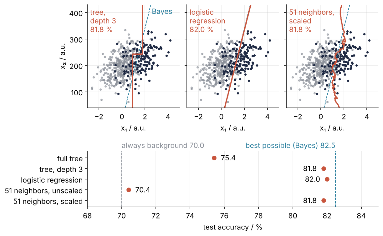
This is where we end up. In each top panel a classifier's decision boundary, the line where its answer flips from background to signal, runs through the 500 test events beside the dashed boundary of the best possible rule. Below them are the test accuracies of five rules between the two numbers above. Tuned honestly, all three methods land within a point of the ceiling, while a tree left to its defaults reaches 75.4 % and the unscaled neighbors 70.4 %. The six steps below build that figure: a split, a decision tree, cross-validation, two more methods, and a pipeline.

Setup

scikit-learn installs with pip install scikit-learn and imports as sklearn. Every model in it takes data in the same layout: a two-dimensional array X with one row per event and one column per feature (a measured quantity), and a one-dimensional array y with one label per row.

import numpy as np
import matplotlib.pyplot as plt
from sklearn.model_selection import train_test_split, cross_val_score
from sklearn.tree import DecisionTreeClassifier
from sklearn.linear_model import LogisticRegression
from sklearn.neighbors import KNeighborsClassifier
from sklearn.preprocessing import StandardScaler
from sklearn.pipeline import make_pipeline
from sklearn.dummy import DummyClassifier

plt.rcParams.update({
    "figure.figsize": (7, 3.6), "figure.dpi": 110,
    "axes.spines.top": False, "axes.spines.right": False,
    "axes.grid": True, "grid.alpha": 0.25,
    "font.size": 11, "lines.linewidth": 1.8,
})
INK, ACCENT, SECOND, MUTED = "#1f2a44", "#c8553d", "#2a7f9e", "#8a8f98"

SEED = 40
mu_signal = np.array([1.6, 220.0])
mu_background = np.array([0.0, 200.0])
cov = np.array([[1.0, 25.0],        # x1 has sd 1, x2 has sd 50,
                [25.0, 2500.0]])    # and their correlation is 25 / (1 * 50) = 0.5

rng = np.random.default_rng(SEED)
X = np.vstack([rng.multivariate_normal(mu_signal, cov, size=600),
               rng.multivariate_normal(mu_background, cov, size=1400)])
y = np.concatenate([np.ones(600, dtype=int), np.zeros(1400, dtype=int)])   # 1 = signal, 0 = background
print(X.shape, y.shape, y.mean())

(2000, 2) (2000,) 0.3

Step 1: Split the data into a training and a test set

A rule judged on the events it learned from looks better than it is, by almost 25 points in Step 2. So a quarter of the events go into a test set that is locked away and scored once, at the end. The other three quarters, the training set, are what every model learns from:

X_train, X_test, y_train, y_test = train_test_split(
    X, y, test_size=0.25, stratify=y, random_state=0)
print(f"training {X_train.shape}, signal fraction {y_train.mean():.3f}")
print(f"test     {X_test.shape}, signal fraction {y_test.mean():.3f}")

training (1500, 2), signal fraction 0.300
test     (500, 2), signal fraction 0.300

stratify=y keeps the signal fraction at 30 % in both sets. The function shuffles before it splits, which matters here because Setup stacked all the signal on top, and random_state=0 fixes that shuffle (Random numbers with numpy.random explains seeds). Plot the training set:

fig, ax = plt.subplots()
bg = y_train == 0
ax.plot(X_train[bg, 0], X_train[bg, 1], "o", ms=3, color=MUTED, alpha=0.6)
ax.plot(X_train[~bg, 0], X_train[~bg, 1], "o", ms=3, color=INK)
ax.text(-2.9, 318, "background", color=MUTED)
ax.text(3.4, 110, "signal", color=INK)
ax.set(xlabel="x₁ / a.u.", ylabel="x₂ / a.u.")
plt.show()

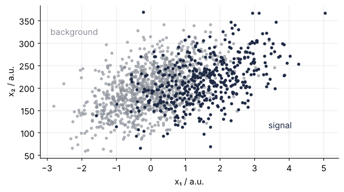
The two clouds overlap, so no rule gets every event right. The tick labels show x₂ spanning about 40 times the range of x₁, which matters in Steps 4 and 5.

Step 2: Fit a decision tree and score it

A decision tree asks a yes-or-no question about one feature, such as "is x₁ < 0.8?", then another question on each side, and keeps splitting until each region, called a leaf, holds events of mostly one class. A new event follows the questions down to a leaf and gets its majority label. The random_state is there because the tree breaks ties between equally good questions at random:

tree = DecisionTreeClassifier(random_state=0)
tree.fit(X_train, y_train)
print("predicted:", tree.predict(X_test[:5]))
print("true:     ", y_test[:5])

predicted: [0 1 0 0 0]
true:      [0 0 0 1 0]

.predict labels new events, and on the first five test events the tree is wrong twice. .score returns the accuracy on any set you hand it:

print(f"accuracy on training {tree.score(X_train, y_train):.3f}, on test {tree.score(X_test, y_test):.3f}")
print(f"depth {tree.get_depth()}, leaves {tree.get_n_leaves()}")

accuracy on training 1.000, on test 0.754
depth 23, leaves 307

A perfect score on the training set and 75.4 % on the test set. With 307 leaves for 1,500 events, the tree has walled off every few training events and memorized the sample, not the populations. That is overfitting. The honest number is 75.4 %, 5 points above always answering background.

Every model in scikit-learn follows this pattern: Model(options), then .fit, .predict, and .score. .fit returns the model itself, so the first two chain into one line. The options are called hyperparameters, settings chosen before fitting rather than learned, and the tree's most important one is max_depth, the longest chain of questions it may ask.

Step 3: Choose the tree depth with cross-validation

The obvious way to choose max_depth is by its test score. Do not: the test set would then have helped choose the model, and its score would no longer be honest. Cross-validation gets the same information from the training set alone: it cuts it into five parts, called folds, and trains on four and scores on the fifth, five times over. cross_val_score returns the five scores:

depths = np.arange(1, 11)
cv_mean, cv_sd, train_acc = [], [], []
for d in depths:
    model = DecisionTreeClassifier(max_depth=d, random_state=0)
    scores = cross_val_score(model, X_train, y_train, cv=5)
    cv_mean.append(scores.mean())
    cv_sd.append(scores.std())
    train_acc.append(model.fit(X_train, y_train).score(X_train, y_train))
    print(f"max_depth {d:2d}   CV {scores.mean():.3f} ± {scores.std():.3f}   training {train_acc[-1]:.3f}")

max_depth  1   CV 0.801 ± 0.022   training 0.802
max_depth  2   CV 0.805 ± 0.020   training 0.802
max_depth  3   CV 0.809 ± 0.014   training 0.825
max_depth  4   CV 0.806 ± 0.016   training 0.826
max_depth  5   CV 0.786 ± 0.023   training 0.838
max_depth  6   CV 0.788 ± 0.011   training 0.852
max_depth  7   CV 0.778 ± 0.026   training 0.866
max_depth  8   CV 0.778 ± 0.024   training 0.876
max_depth  9   CV 0.775 ± 0.024   training 0.891
max_depth 10   CV 0.766 ± 0.030   training 0.907

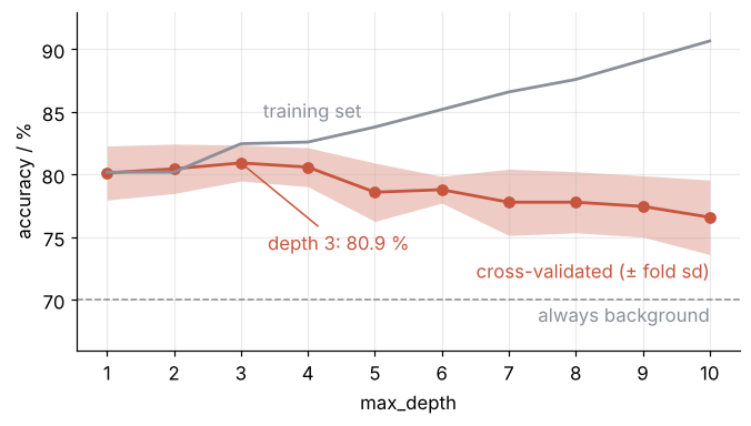
Training accuracy climbs from 80.2 % to 90.7 %. The cross-validated accuracy peaks at depth 3 with 80.9 % and falls to 76.6 % by depth 10, as each further level fits more noise. The spread over the folds is about 1.5 points, so the decimal is noise: depth 3 against depth 4, 80.9 against 80.6, is a tie, and you take the smaller tree, which has less room to fit noise.

cv_mean, cv_sd, train_acc = 100 * np.array(cv_mean), 100 * np.array(cv_sd), 100 * np.array(train_acc)
fig, ax = plt.subplots()
ax.fill_between(depths, cv_mean - cv_sd, cv_mean + cv_sd, color=ACCENT, alpha=0.30, lw=0)
ax.plot(depths, cv_mean, "o-", color=ACCENT, ms=6)
ax.plot(depths, train_acc, color=MUTED)
ax.text(4.8, 84.2, "training set", color=MUTED, ha="right", va="bottom")
ax.text(10, 73.2, "cross-validated (± fold sd)", color=ACCENT, ha="right", va="top")
ax.axhline(70, color=MUTED, ls="--", lw=1)
ax.text(10, 69.7, "always background", color=MUTED, ha="right", va="top")
ax.annotate(f"depth 3: {cv_mean[2]:.1f} %", xy=(3, cv_mean[2]), xytext=(3.4, 74),
            color=ACCENT, arrowprops=dict(arrowstyle="-", color=ACCENT, lw=1))
ax.set(xlabel="max_depth", ylabel="accuracy / %", xticks=depths, ylim=(66, 93))
plt.show()

Refit at depth 3 on the whole training set and score the test set, once:

tree3 = DecisionTreeClassifier(max_depth=3, random_state=0).fit(X_train, y_train)
print(f"depth 3: test accuracy {tree3.score(X_test, y_test):.3f}, {tree3.get_n_leaves()} leaves")

depth 3: test accuracy 0.818, 8 leaves

81.8 % from eight leaves: 6 points better than the tree with 307, and within a point of the ceiling.

Step 4: Fit a logistic regression

A second method, the same calls. Logistic regression computes a weighted sum of the features, which is zero along a straight line in the plane, positive on one side and negative on the other, and passes the sum through the logistic function \(1/(1 + e^{-z})\), which squashes any number into a probability between 0 and 1. An event on the positive side gets a signal probability above 0.5 and is called signal, so the line is the decision boundary.

logreg = LogisticRegression().fit(X_train, y_train)
print(f"test accuracy {logreg.score(X_test, y_test):.3f}")
print("P(background), P(signal) of three test events:")
print(logreg.predict_proba(X_test[:3]).round(3))
w1, w2 = logreg.coef_[0]
print(f"weights: x1 {w1:.3f}, x2 {w2:.4f}")

test accuracy 0.820
P(background), P(signal) of three test events:
[[0.978 0.022]
 [0.774 0.226]
 [0.766 0.234]]
weights: x1 1.717, x2 -0.0100

82.0 %, with the default options and no tuning. That is no accident: for two Gaussian populations with the same covariance, the best possible boundary is itself a straight line, the shape this method draws. predict_proba returns one column per class, background first. coef_ holds the weights, and a trailing underscore marks anything .fit learned from the data. The weight of x₂ is about 170 times smaller than that of x₁, which reflects the units of x₂, not its importance: in units 50 times larger, x₂ would get a weight 50 times larger and, to a good approximation, the same line. The tree is just as indifferent, because a threshold on x₂ splits the same events in any unit.

Step 5: Put a scaler in front of nearest neighbors with a pipeline

Nearest neighbors labels an event by majority vote among the k training events closest to it, and k is its hyperparameter. Closest means the Euclidean distance \(\sqrt{\Delta x_1^2 + \Delta x_2^2}\), which adds up the differences in both features, and there the units bite. One standard deviation of x₂ is 50 units against 1 for x₁, so the neighbors are chosen almost by x₂ alone. StandardScaler fixes this, and belongs in front of every method built on distances between events: it subtracts each feature's training mean and divides by its training standard deviation, so both features count equally.

make_pipeline chains the scaler and the classifier into one model with the same .fit and .score. It goes into cross_val_score whole, so in each round the scaler learns from the four training folds only. Scale the training set once beforehand instead, and the fold being scored has already shaped the model, the leak Step 3 warned about. The raw classifier runs alongside:

print("    k    raw   scaled")
for k in [1, 5, 15, 25, 51, 101]:
    raw = cross_val_score(KNeighborsClassifier(n_neighbors=k), X_train, y_train, cv=5).mean()
    pipe = make_pipeline(StandardScaler(), KNeighborsClassifier(n_neighbors=k))
    scaled = cross_val_score(pipe, X_train, y_train, cv=5).mean()
    print(f"{k:5d}  {raw:.3f}  {scaled:.3f}")

    k    raw   scaled
    1  0.724  0.740
    5  0.764  0.794
   15  0.738  0.801
   25  0.721  0.815
   51  0.703  0.817
  101  0.700  0.814

The scaled column rises from 74.0 % at k = 1 to 81.7 % at k = 51 and dips at 101. The raw column peaks at 76.4 % for k = 5 and sinks to 70.3 % at k = 51, the always-background level: 51 neighbors picked by x₂ alone are mostly background. Take k = 51 from the scaled column, fit, and score once:

knn = make_pipeline(StandardScaler(), KNeighborsClassifier(n_neighbors=51)).fit(X_train, y_train)
print(f"k = 51: test accuracy {knn.score(X_test, y_test):.3f}")
mean, sd = knn[0].mean_, knn[0].scale_
print(f"scaler mean: x1 {mean[0]:.2f}, x2 {mean[1]:.2f}")
print(f"scaler sd:   x1 {sd[0]:.2f}, x2 {sd[1]:.2f}")

k = 51: test accuracy 0.818
scaler mean: x1 0.49, x2 204.34
scaler sd:   x1 1.20, x2 51.31

81.8 %, the same as the tuned tree. A pipeline indexes like a list, so knn[0] is the scaler. Its standard deviations, 1.20 for x₁ and 51.31 for x₂, come from the training set only and exceed Setup's 1 and 50 because the pooled populations are wider than either.

Step 6: Compare with the best possible rule

The data come from two known Gaussians, so the best possible rule can be written down. It is Bayes' rule: call an event signal when 0.3 times the signal density at that point exceeds 0.7 times the background density. The 0.3 and 0.7 are the priors, the class fractions you would bet on before measuring anything. The collapsed cell builds it with scipy.stats.multivariate_normal and scores it on a million fresh events, enough to pin the ceiling down, and on the 500 test events:

Show code

from scipy.stats import multivariate_normal

p_signal = multivariate_normal(mu_signal, cov)
p_background = multivariate_normal(mu_background, cov)

def bayes_rule(X):
    return (0.3 * p_signal.pdf(X) > 0.7 * p_background.pdf(X)).astype(int)

rng_fresh = np.random.default_rng(SEED + 1)
n_signal = rng_fresh.binomial(10**6, 0.3)
X_fresh = np.vstack([rng_fresh.multivariate_normal(mu_signal, cov, size=n_signal),
                     rng_fresh.multivariate_normal(mu_background, cov, size=10**6 - n_signal)])
y_fresh = np.concatenate([np.ones(n_signal, dtype=int), np.zeros(10**6 - n_signal, dtype=int)])

acc_ceiling = np.mean(bayes_rule(X_fresh) == y_fresh)
print(f"Bayes rule, 10^6 fresh events: {acc_ceiling:.3f}")
print(f"Bayes rule, the 500 test events: {np.mean(bayes_rule(X_test) == y_test):.3f}")

Bayes rule, 10^6 fresh events: 0.825
Bayes rule, the 500 test events: 0.818

The ceiling is 82.5 %. For the floor, DummyClassifier ignores the features and always answers the most frequent class. The unscaled neighbors are fitted only now, after every choice is made:

floor = DummyClassifier(strategy="most_frequent").fit(X_train, y_train)
knn_raw = KNeighborsClassifier(n_neighbors=51).fit(X_train, y_train)
results = {"full tree": tree, "tree, depth 3": tree3, "logistic regression": logreg,
           "51 neighbors, unscaled": knn_raw, "51 neighbors, scaled": knn}
acc_floor = floor.score(X_test, y_test)
print(f"{'always background':24s} {acc_floor:.3f}")
for name, model in results.items():
    print(f"{name:24s} {model.score(X_test, y_test):.3f}")

always background        0.700
full tree                0.754
tree, depth 3            0.818
logistic regression      0.820
51 neighbors, unscaled   0.704
51 neighbors, scaled     0.818

x1g, x2g = np.meshgrid(np.linspace(-3, 5, 300), np.linspace(40, 430, 300))
grid = np.column_stack([x1g.ravel(), x2g.ravel()])
on_grid = lambda rule: rule(grid).reshape(x1g.shape)

fig = plt.figure(figsize=(8, 5.6))
gs = fig.add_gridspec(2, 3, height_ratios=[2.6, 1.4], hspace=0.55, wspace=0.08)
maps = [("tree,\ndepth 3", tree3), ("logistic\nregression", logreg), ("51 neighbors,\nscaled", knn)]
first = None
for i, (name, model) in enumerate(maps):
    ax = fig.add_subplot(gs[0, i], sharex=first, sharey=first)
    first = first or ax
    bg = y_test == 0
    ax.plot(X_test[bg, 0], X_test[bg, 1], "o", ms=2.5, color=MUTED, alpha=0.6)
    ax.plot(X_test[~bg, 0], X_test[~bg, 1], "o", ms=2.5, color=INK)
    ax.contour(x1g, x2g, on_grid(bayes_rule), levels=[0.5], colors=SECOND, linewidths=1, linestyles="--")
    ax.contour(x1g, x2g, on_grid(model.predict), levels=[0.5], colors=ACCENT, linewidths=1.8)
    ax.text(0.03, 0.97, f"{name}\n{100 * model.score(X_test, y_test):.1f} %",
            transform=ax.transAxes, va="top", color=ACCENT)
    ax.set(xlabel="x₁ / a.u.", xticks=[-2, 0, 2, 4], ylim=(40, 430))
    if i == 0:
        ax.set(ylabel="x₂ / a.u.")
        ax.text(2.6, 405, "Bayes", color=SECOND, va="center")
    else:
        ax.tick_params(labelleft=False)

ax = fig.add_subplot(gs[1, :])
names = list(results)
acc = np.array([100 * m.score(X_test, y_test) for m in results.values()])
rows = np.arange(len(names))[::-1]
ax.plot(acc, rows, "o", ms=6, color=ACCENT)
for a, r in zip(acc, rows):
    left = a > 78           # keep the value clear of the ceiling line
    ax.text(a + (-0.4 if left else 0.4), r, f"{a:.1f}", va="center", ha="right" if left else "left")
for level, color, label, side in [(100 * acc_ceiling, SECOND, f"best possible (Bayes) {100 * acc_ceiling:.1f}", "right"),
                                  (100 * acc_floor, MUTED, f"always background {100 * acc_floor:.1f}", "left")]:
    ax.axvline(level, color=color, ls="--", lw=1)
    ax.text(level, 1.03, label, color=color, ha=side, va="bottom",
            transform=ax.get_xaxis_transform(), clip_on=False)
ax.set(yticks=rows, yticklabels=names, xlim=(68, 85), ylim=(-0.6, rows.max() + 0.6),
       xlabel="test accuracy / %")
ax.grid(axis="y", visible=False)
plt.show()

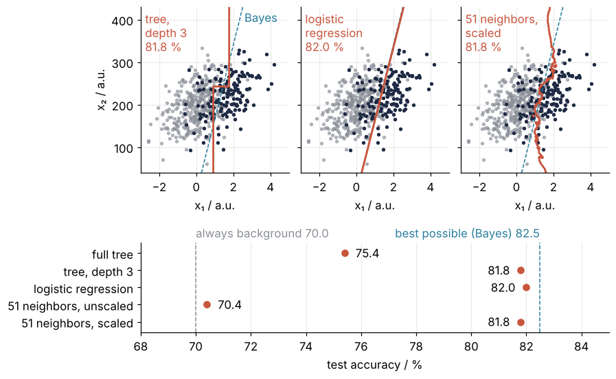
The tuned tree's eight boxes merge into a boundary with one step, logistic regression lies almost on the dashed Bayes line, and the scaled neighbors' wavy line crosses it several times where the events are dense and parts from it below x₂ ≈ 150 and above 330, where few events are left to vote. A fraction measured on 500 events has a standard error, the typical scatter between samples of 500, of \(\sqrt{0.82 \cdot 0.18 / 500} \approx 1.7\) points (scipy.stats from the ground up treats such uncertainties). So 81.8 against 82.0 is a tie, and so is either against the ceiling: the perfect rule itself scores 81.8 on these events.

Pitfalls

Choosing on the test set. Pick max_depth by its test score instead of by cross-validation and you get this:

test_acc = [DecisionTreeClassifier(max_depth=d, random_state=0).fit(X_train, y_train).score(X_test, y_test)
            for d in depths]
print("test accuracy by depth:", " ".join(f"{a:.3f}" for a in test_acc))
print("best on the test set: depth", depths[np.argmax(test_acc)])

test accuracy by depth: 0.824 0.824 0.818 0.816 0.810 0.812 0.806 0.808 0.798 0.774
best on the test set: depth 1

A single question wins with 82.4 %, ahead of the true Bayes rule on the same 500 events (81.8 %). One question cannot beat the best possible rule in the long run; the excess is luck, found by looking at one test set ten times. Every look at the test set that changes a choice turns it into training data, and the same leak happens more quietly when you fit a scaler on all 2,000 events before splitting. Cross-validate on the training set, touch the test set once, and keep preprocessing inside a pipeline as in Step 5.

An unseeded split. The same code on the same data reports a different accuracy on every run. Here is the spread over 20 different splits:

lr_acc, tree_acc = [], []
for seed in range(20):
    Xa, Xb, ya, yb = train_test_split(X, y, test_size=0.25, stratify=y, random_state=seed)
    lr_acc.append(LogisticRegression().fit(Xa, ya).score(Xb, yb))
    tree_acc.append(DecisionTreeClassifier(random_state=0).fit(Xa, ya).score(Xb, yb))
print(f"logistic regression {min(lr_acc):.3f} to {max(lr_acc):.3f}")
print(f"full tree           {min(tree_acc):.3f} to {max(tree_acc):.3f}")

logistic regression 0.798 to 0.836
full tree           0.694 to 0.768

Logistic regression moves between 79.8 % and 83.6 %, the upper end above the ceiling, which is what a 1.7-point standard error does. The full tree moves between 69.4 % and 76.8 %. train_test_split shuffles at random, and so does the tree when two questions are equally good. Pass random_state= to both, and when you report a number, quote the cross-validated mean with its fold spread rather than the third digit of one split.

An accuracy without its baseline. 70.4 % sounds like a classifier that works, until you remember that answering background every time gets 70.0 % (the unscaled neighbors in Step 6). With unequal classes, accuracy has a floor far above 50 %. Score a DummyClassifier next to every model, split with stratify so the test set keeps the class ratio, and when signal is what you are after, look at it on its own. confusion_matrix counts, for each true class (rows: background, signal), how many events were labeled background and how many signal (columns):

from sklearn.metrics import confusion_matrix
print(confusion_matrix(y_test, knn_raw.predict(X_test)))

[[350   0]
 [148   2]]

The unscaled neighbors call two of the 150 signal events signal. As a signal detector it is nearly blind.

Variations

GridSearchCV replaces the loops of Steps 3 and 5. GridSearchCV(model, {"max_depth": range(1, 11)}, cv=5).fit(X_train, y_train) searches, refits the best model on the whole training set, and reports the choice in best_params_. For a pipeline, a parameter is named <step>__<parameter> with two underscores, as in {"kneighborsclassifier__n_neighbors": [5, 25, 51]}; make_pipeline names each step after its class in lowercase.
A threshold instead of a label. .predict calls an event signal when its signal probability exceeds 0.5. Use predict_proba(X)[:, 1] > t instead: a higher t calls fewer background events signal and misses more true signal, a lower t the reverse. TunedThresholdClassifierCV in sklearn.model_selection chooses t by cross-validation for the trade-off you name.
Forests and boosting. RandomForestClassifier and HistGradientBoostingClassifier from sklearn.ensemble drop into the same calls. With messier boundaries than these two Gaussians, they usually beat a single tree.
Regression. To predict a number instead of a class, use DecisionTreeRegressor, KNeighborsRegressor, or LinearRegression; .score then reports R² instead of accuracy.

Cheat sheet

X_train, X_test, y_train, y_test = train_test_split(X, y, test_size=0.25, stratify=y, random_state=0)
model = DecisionTreeClassifier(max_depth=3, random_state=0)  # options are hyperparameters
model.fit(X_train, y_train)                                  # learns; attributes ending in _ come from here
model.predict(X_new), model.predict_proba(X_new)             # labels; one probability column per class
cross_val_score(model, X_train, y_train, cv=5).mean()        # choose hyperparameters with this
pipe = make_pipeline(StandardScaler(), KNeighborsClassifier(n_neighbors=51))  # scaler refitted per fold
DummyClassifier(strategy="most_frequent").fit(X_train, y_train)               # the floor to compare with
confusion_matrix(y_test, model.predict(X_test))              # rows true class, columns predicted
model.score(X_test, y_test)                                  # once, at the very end