PCA with MultivariateStats.jl: sixty absorption spectra in two dimensions

The problem: 6,000 absorbances from three compounds

Sixty samples sit on your bench, 20 of each of three compounds, and you have recorded a UV-Vis absorption spectrum of every one at 100 wavelengths from 250 to 646 nm. That makes a 60 × 100 table, a row per sample. Nobody can draw 100 axes, and a pair of wavelengths chosen by hand tells the compounds apart only when you know beforehand where their bands lie. Principal component analysis (PCA) replaces the wavelengths with new axes, the directions through the 100-dimensional space in which the samples vary most, and MultivariateStats.jl fits them. Gene expression profiles, metabolite panels, and element concentrations in rocks arrive as tables of the same shape, and what follows applies to them unchanged.

MultivariateStats and StatsBase expect each sample in a column, so the matrix here is 100 × 60, wavelengths down and spectra across. The spectra are generated, so that their contents are known, with the recipe of the Python version of this tutorial; Julia's random numbers are not NumPy's, so each number below differs slightly from its counterpart there. Every compound contributes three absorption bands, and four things change between samples. A concentration factor multiplies the entire spectrum and varies by about 8 %. Band heights vary by 5 % and band positions by 2 nm. Each absorbance carries 0.01 units of noise, and each spectrum a small shift of its baseline.

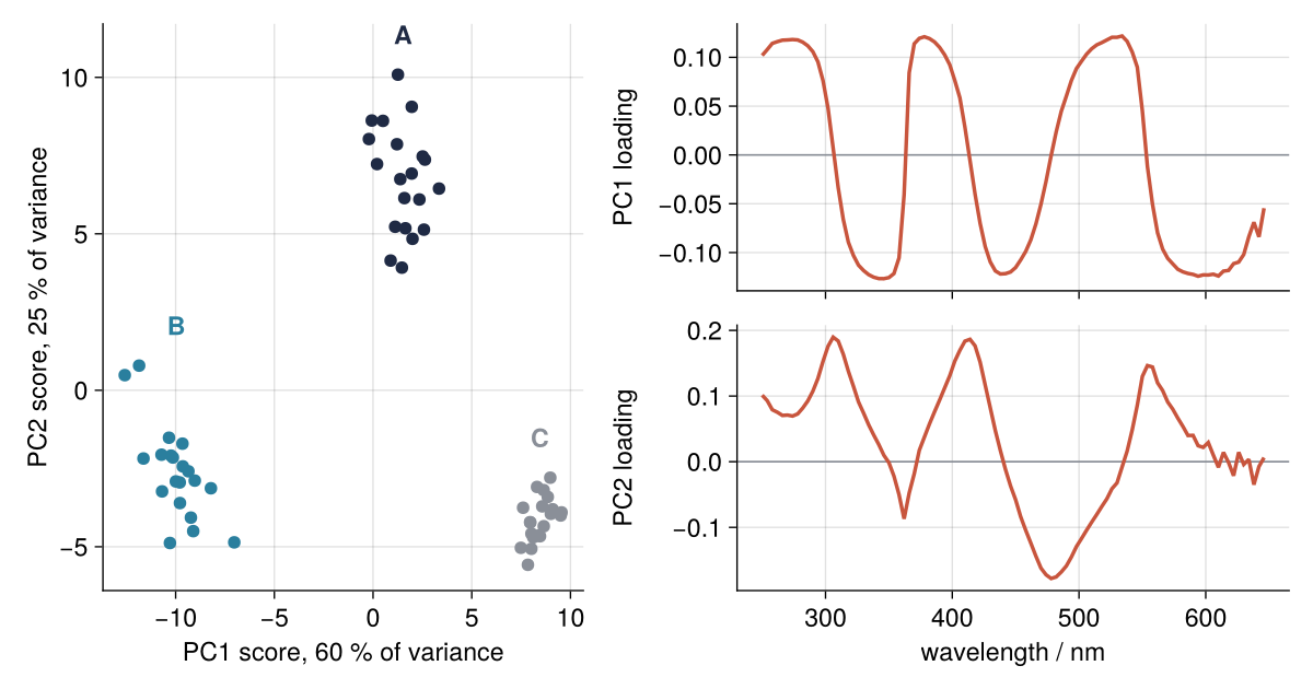
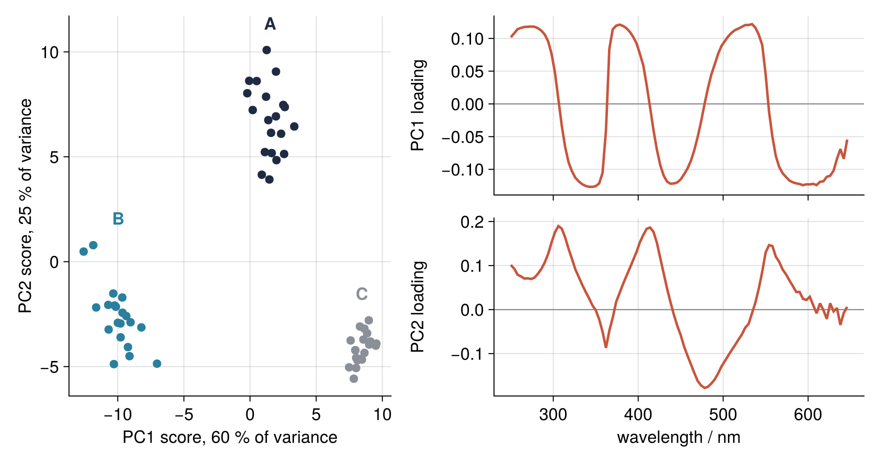
Left: scores of 60 spectra on the first two principal components, PC2 (25 % of the variance) against PC1 (60 %), in three separate clusters for compounds A, B, and C. Right: the PC1 and PC2 loadings against wavelength in nm, which switch sign at the bands where the compounds differ.

That is the destination. In the left panel each dot is a spectrum, positioned by its coordinates on the first two directions PCA found. The 60 samples form three clusters, one per compound, and PCA never saw a label. Together the two directions hold 84.9 % of the variation. In the right panel the loadings give the weight of each wavelength in each direction, and they single out the bands where the compounds disagree. Five steps build it.

Setup

Install the packages once with import Pkg; Pkg.add(["MultivariateStats", "StatsBase", "CairoMakie"]); Statistics, LinearAlgebra, Random, and Printf ship with Julia. Both MultivariateStats and StatsBase define a function transform, and they are different functions, so the code below writes StatsBase.transform and StatsBase.reconstruct to say whose they are; fit and predict need no prefix, because MultivariateStats adds its methods to the StatsBase functions of those names instead of defining its own. A fresh session spends a minute or so compiling CairoMakie; the computations take well under a second.

using MultivariateStats, StatsBase, Statistics, LinearAlgebra, Random, Printf, CairoMakie

const INK, ACCENT, SECOND, MUTED = "#1f2a44", "#c8553d", "#2a7f9e", "#8a8f98"
set_theme!(Theme(
    size = (770, 396), fontsize = 17,
    palette = (color = [INK, ACCENT, SECOND, MUTED],),
    Axis = (topspinevisible = false, rightspinevisible = false, xgridvisible = true, ygridvisible = true),
    Lines = (linewidth = 2.5,),
))
const COMPOUNDS = ["A" => INK, "B" => SECOND, "C" => MUTED]

const SEED = 85
const wavelength = 250.0:4:646                         # nm, 100 rows
const BANDS = Dict(                                    # (center / nm, width / nm, height / absorbance)
    "A" => [(300, 25, 0.8), (420, 30, 0.5), (540, 35, 0.3)],
    "B" => [(320, 25, 0.6), (450, 30, 0.7), (560, 35, 0.25)],
    "C" => [(290, 20, 0.7), (400, 30, 0.3), (500, 40, 0.6)],
)

function make_spectra(; conc_sd = 0.08, n_per = 20, seed = SEED)
    rng = Xoshiro(seed)
    X = zeros(length(wavelength), 0)
    compound, conc = String[], Float64[]
    for (name, _) in COMPOUNDS, _ in 1:n_per
        c = exp(conc_sd * randn(rng))                  # concentration factor, lognormal, always positive
        a = zeros(length(wavelength))
        for (center, width, height) in BANDS[name]
            h = height * (1 + 0.05 * randn(rng))
            shift = 2 * randn(rng)
            @. a += h * exp(-0.5 * ((wavelength - center - shift) / width)^2)
        end
        a = c .* a .+ 0.01 .* randn(rng, length(wavelength)) .+ 0.005 * randn(rng)
        X = hcat(X, a)
        push!(compound, name)
        push!(conc, c)
    end
    return X, compound, conc
end

X, compound, conc = make_spectra()                     # your own matrix goes here: rows variables, columns samples
println("X: $(size(X, 1)) wavelengths × $(size(X, 2)) samples, compounds ", join(first.(COMPOUNDS), ", "))

X: 100 wavelengths × 60 samples, compounds A, B, C

Step 1: Look at the raw spectra and at one pair of wavelengths

First the plain view: every spectrum in one panel, and beside it the absorbance at one wavelength over that at another.

picked = [302, 450]                                    # nm, chosen by eye
rows = [findfirst(==(w), wavelength) for w in picked]

fig = Figure(size = (880, 374))
ax1 = Axis(fig[1, 1], xlabel = "wavelength / nm", ylabel = "absorbance")
ax2 = Axis(fig[1, 2], xlabel = "absorbance at $(picked[1]) nm", ylabel = "absorbance at $(picked[2]) nm")
for (name, color) in COMPOUNDS
    s = compound .== name
    for k in findall(s)
        lines!(ax1, wavelength, X[:, k], color = (color, 0.5), linewidth = 1.4)
    end
    scatter!(ax2, X[rows[1], s], X[rows[2], s], color = color, markersize = 8)
    text!(ax2, mean(X[rows[1], s]), maximum(X[rows[2], s]) + 0.02, text = name,
          color = color, align = (:center, :bottom), font = :bold)
end
vlines!(ax1, picked, color = MUTED, linewidth = 1.2, linestyle = :dash)
ylims!(ax2, 0.2, 1.05)                                 # room for the label above B
display(fig)

for (name, _) in COMPOUNDS
    s = compound .== name
    println(name, "  ", join([@sprintf("%d nm: %.2f to %.2f", w, extrema(X[j, s])...) for (w, j) in zip(picked, rows)], "   "))
end

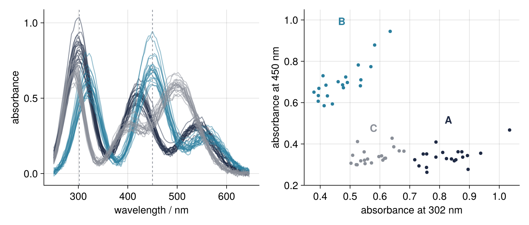
Left: 60 absorption spectra, absorbance against wavelength in nm, colored by compound, overlapping heavily; dashed lines mark 302 and 450 nm. Right: absorbance at 450 nm against absorbance at 302 nm. B stands apart; A and C share the range at 450 nm and nearly touch at 302 nm.

A  302 nm: 0.72 to 1.03   450 nm: 0.26 to 0.47
B  302 nm: 0.38 to 0.63   450 nm: 0.59 to 0.94
C  302 nm: 0.50 to 0.68   450 nm: 0.30 to 0.43

Outside the region around 450 nm the spectra lie on top of each other; there B absorbs far more than the others and stands clear in the scatter. At 450 nm, A and C overlap between 0.30 and 0.43. At 302 nm they barely come apart, A from 0.72 upward and C at most 0.68, a gap of 0.04. This pair works only because I chose it after seeing the bands, and 100 wavelengths make 4,950 possible pairs. PCA skips the choice and makes every new axis out of all 100 wavelengths together.

Step 2: Standardize the wavelengths with ZScoreTransform

PCA ranks directions by how far the samples scatter along them, so anything that inflates a wavelength's scatter inflates its weight too. Standardizing evens this out: it subtracts each row's mean (centering) and divides by the row's standard deviation (scaling), leaving every wavelength at mean 0 and standard deviation 1.

dt = fit(ZScoreTransform, X; dims = 2)
Z = StatsBase.transform(dt, X)

println("wavelength    mean     scale   |  mean after  sd after")
for w in [302, 450, 562, 646]
    j = findfirst(==(w), wavelength)
    @printf("%6d nm  %7.3f  %7.4f   |  %10.1e  %8.3f\n", w, dt.mean[j], dt.scale[j], mean(Z[j, :]), std(Z[j, :]))
end

wavelength    mean     scale   |  mean after  sd after
   302 nm    0.627   0.1658   |     3.4e-16     1.000
   450 nm    0.460   0.1825   |    -3.5e-17     1.000
   562 nm    0.227   0.0419   |     8.8e-16     1.000
   646 nm    0.005   0.0109   |     3.5e-17     1.000

fit takes a type and the data and returns a fitted object, dt, which stores what it learned: one mean and one standard deviation per wavelength, in the fields dt.mean and dt.scale. StatsBase.transform(dt, X) applies them, to these spectra or to new ones. PCA follows the same pattern, fit in Step 3 and predict in Step 4.

dims = 2 computes them along the second dimension, over the samples, one pair per row; the first pitfall shows dims = 1. Unscaled, the absorbance at 302 nm varies by 0.166 units between samples, and at 646 nm, where no compound absorbs, by 0.011, which is the noise. Scaled, both vary by exactly 1, because StatsBase and std both divide by n − 1. Now the faint band at 562 nm weighs the same as the strong one at 302 nm, which is what you want, and so does every empty wavelength, which is the price.

Standardize without exception when the variables come in different units or at very different sizes, temperatures next to concentrations. When they share a unit and a noise level, as the points of a spectrum do, spectroscopists usually only center, which leaves the strong bands strong and the empty regions silent: hand X directly to fit(PCA, X), which centers it. I standardize here because that works for any matrix; Steps 4 and 5 show what centering alone does to this one.

Step 3: Fit PCA and decide how many components to keep

Think of a direction as a unit vector w holding 100 weights, one for each wavelength. A sample's coordinate along it is the weighted sum dot(Z[:, i], w), and the variance of the 60 coordinates is the variance in that direction. The 100 row variances add up to the total. The first principal component (PC1) is the direction with the most variance; PC2 has the most among the directions at right angles to PC1, and so on, up to 59: centered, the 60 spectra sum to zero, so any one follows from the rest. The component variances sum to the total.

M = fit(PCA, Z; pratio = 1.0)                          # keep every component, for the plot below
ratio = principalvars(M) ./ var(M)

@printf("largest entry of mean(M): %.1e\n", maximum(abs, mean(M)))
@printf("components kept: %d, total variance var(M) = %.2f\n", size(M, 2), var(M))
println("share of variance / %: ", round.(100 .* ratio[1:6]; digits = 1))
println("cumulative / %:        ", round.(100 .* cumsum(ratio[1:6]); digits = 1))

w1 = projection(M)[:, 1]                               # PC1 as a unit vector
@printf("PC1 by the definition: %.4f   MultivariateStats: %.4f\n", var(Z' * w1) / sum(var(Z; dims = 2)), ratio[1])

largest entry of mean(M): 2.4e-15
components kept: 59, total variance var(M) = 100.00
share of variance / %: [59.5, 25.4, 6.3, 1.5, 1.1, 1.0]
cumulative / %:        [59.5, 84.9, 91.2, 92.7, 93.8, 94.8]
PC1 by the definition: 0.5952   MultivariateStats: 0.5952

M holds four things you read with functions: mean(M), the means it subtracts before projecting, zero to rounding since Z is centered; projection(M), the directions; principalvars(M), the variance along each; and var(M), the total, here 100.00, since each of the 100 rows has variance 1. Both sides of the hand check divide by n − 1, as var does by default, and agree at 0.5952. Without pratio = 1.0, fit stops once the kept components reach 99 % of the variance.

k = 1:10
fig = Figure(size = (770, 374))
ax = Axis(fig[1, 1], xlabel = "principal component", ylabel = "share of variance / %", xticks = k)
lines!(ax, k, 100 .* cumsum(ratio[k]), color = (INK, 0.6), linewidth = 1.6)
text!(ax, 10, 100 * sum(ratio[k]) - 7, text = "cumulative", color = (INK, 0.8), align = (:right, :center))
scatter!(ax, k, 100 .* ratio[k], color = INK, markersize = 12)
for i in 1:3
    text!(ax, k[i] + 0.25, 100 * ratio[i], text = @sprintf("%.1f %%", 100 * ratio[i]), align = (:left, :center))
end
hlines!(ax, [100 * ratio[4]], color = MUTED, linewidth = 1.2, linestyle = :dash)
text!(ax, 10, 100 * ratio[4] + 3, text = "noise floor", color = MUTED, align = (:right, :bottom))
ylims!(ax, -3, 100)                                    # room below the dots on the floor
display(fig)

@printf("pratio = 0.99 (default) keeps %d components, pratio = 0.95 keeps %d, maxoutdim = 3 keeps %d\n",
        size(fit(PCA, Z), 2), size(fit(PCA, Z; pratio = 0.95), 2), size(fit(PCA, Z; maxoutdim = 3), 2))

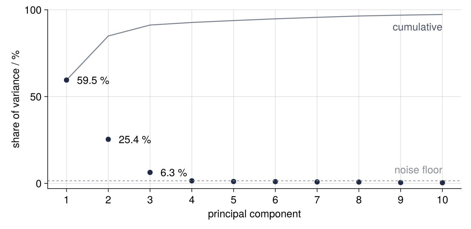
Share of the variance in % for principal components 1 to 10. Dots: 59.5, 25.4, and 6.3 % for the first three, then a flat floor below 2 %. Line: the cumulative share, reaching 91 % at three components.

pratio = 0.99 (default) keeps 19 components, pratio = 0.95 keeps 7, maxoutdim = 3 keeps 3

PC1 holds 59.5 %, PC2 25.4 %, PC3 6.3 %, and every later component stays below 2 %, a level floor made of noise. Keep what stands above the floor, up to the elbow where the curve bends flat, and ignore any fixed percentage. That gives three here, exactly what maxoutdim = 3 keeps. The default keeps 19, and pratio = 0.95 keeps seven, four of which are noise. Step 4 plots only two, since two already separate the compounds.

Step 4: Project the samples and color the scores by compound

M is now applied like dt in Step 2. predict returns the scores, every sample's coordinates on every component, Step 3's projections all at once:

S = predict(M, Z)
println(size(S), "  ", S ≈ projection(M)' * (Z .- mean(M)))

(59, 60)  true

One row per component, one column per sample. Plotted against each other and colored by labels that PCA never saw:

score_label(i) = @sprintf("PC%d score, %.0f %% of variance", i, 100 * ratio[i])

fig = Figure(size = (605, 495))
ax = Axis(fig[1, 1], xlabel = score_label(1), ylabel = score_label(2), autolimitaspect = 1)
for (name, color) in COMPOUNDS
    s = compound .== name
    scatter!(ax, S[1, s], S[2, s], color = color, markersize = 12)
    text!(ax, mean(S[1, s]), maximum(S[2, s]) + 0.8, text = name, color = color, align = (:center, :bottom), font = :bold)
end
display(fig)

for (name, _) in COMPOUNDS
    s = compound .== name
    @printf("%s: center PC1 %+6.2f   PC2 %+6.2f\n", name, mean(S[1, s]), mean(S[2, s]))
end

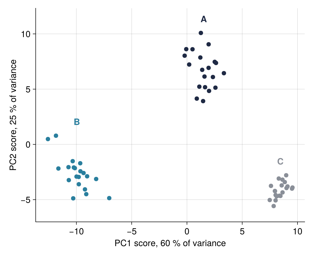
Scores of 60 spectra, PC2 against PC1. Three separate clusters: B on the left along PC1, C on the right, A in the middle and above both along PC2.

A: center PC1  +1.52   PC2  +6.76
B: center PC1  -9.96   PC2  -2.62
C: center PC1  +8.45   PC2  -4.13

Three clusters, well apart. PC1 puts B (centered at −9.96) and C (+8.45) at opposite ends with A between, and PC2 raises A (+6.76) above both. The third component belongs to no compound; its scores track the concentration factor:

for i in 1:4
    @printf("PC%d: correlation with concentration r = %+.2f\n", i, cor(S[i, :], conc))
end

PC1: correlation with concentration r = -0.05
PC2: correlation with concentration r = +0.40
PC3: correlation with concentration r = +0.77
PC4: correlation with concentration r = +0.18

The correlation coefficient r would be +1 if the scores grew exactly in step with the concentration, and 0 if they paid it no attention. PC3 reaches 0.77, PC2 picks up some with 0.40, and PC1 and PC4 stay below 0.2. A component may stand for a physical effect rather than a substance.

New samples go through the fitted dt and M, never a refit, so that they land on the same map. Three fresh spectra:

X_new, compound_new, _ = make_spectra(n_per = 1, seed = SEED + 2)
S_new = predict(M, StatsBase.transform(dt, X_new))
for (k, name) in enumerate(compound_new)
    @printf("%s: PC1 %+6.2f   PC2 %+6.2f\n", name, S_new[1, k], S_new[2, k])
end

A: PC1  +0.53   PC2  +4.14
B: PC1  -9.33   PC2  -3.53
C: PC1  +8.65   PC2  -2.74

Each falls into its own cluster, C at the top edge. Step 2 still owes the PCA of centered-only spectra:

Mc = fit(PCA, X; pratio = 1.0)
Sc = predict(Mc, X)
ratio_c = principalvars(Mc) ./ var(Mc)
@printf("centered only: PC1 %.1f %%, PC2 %.1f %%, together %.1f %% (standardized: %.1f %%)\n",
        100 * ratio_c[1], 100 * ratio_c[2], 100 * sum(ratio_c[1:2]), 100 * sum(ratio[1:2]))
for (name, _) in COMPOUNDS
    s = compound .== name
    @printf("%s: PC1 %+.2f ± %.2f   PC2 %+.2f ± %.2f\n", name, mean(Sc[1, s]), std(Sc[1, s]), mean(Sc[2, s]), std(Sc[2, s]))
end

centered only: PC1 58.4 %, PC2 33.6 %, together 92.0 % (standardized: 84.9 %)
A: PC1 +0.21 ± 0.12   PC2 +1.01 ± 0.14
B: PC1 -1.26 ± 0.14   PC2 -0.37 ± 0.11
C: PC1 +1.06 ± 0.08   PC2 -0.64 ± 0.07

The cluster centers are about 2 apart, in absorbance rather than standard deviations, and no cluster is wider than 0.14: as clean a separation as before. PC1 and PC2 hold 92.0 % instead of 84.9 %. That is no better fit: unscaled, the empty wavelengths add almost nothing to the total, so a share means something only next to shares from the same preprocessing.

Step 5: Interpret the loadings and assemble the final figure

MultivariateStats has two functions for loadings. projection(M) returns the unit vectors w of Step 3, one column per component: what chemometrics calls loadings, and what this step plots. loadings(M) scales each column by the square root of its component's variance; it comes in at the end.

P = projection(M)
@printf("size %s, length of column 1: %.6f\n", size(P), norm(P[:, 1]))

means = Dict(name => vec(mean(X[:, compound .== name]; dims = 2)) for (name, _) in COMPOUNDS)
println("\nwavelength   mean A   mean B   mean C  |  PC1 loading  PC2 loading")
for w in [270, 306, 338, 378, 414, 450, 478, 526, 622]
    j = findfirst(==(w), wavelength)
    @printf("%6d nm  %7.2f  %7.2f  %7.2f  |  %+11.3f  %+11.3f\n", w, means["A"][j], means["B"][j], means["C"][j], P[j, 1], P[j, 2])
end

size (100, 59), length of column 1: 1.000000

wavelength   mean A   mean B   mean C  |  PC1 loading  PC2 loading
   270 nm     0.40     0.09     0.42  |       +0.118       +0.071
   306 nm     0.81     0.52     0.50  |       +0.007       +0.190
   338 nm     0.28     0.45     0.08  |       -0.125       +0.041
   378 nm     0.20     0.08     0.24  |       +0.121       +0.037
   414 nm     0.51     0.36     0.33  |       -0.006       +0.186
   450 nm     0.34     0.70     0.34  |       -0.115       -0.058
   478 nm     0.15     0.46     0.52  |       -0.001       -0.178
   526 nm     0.29     0.18     0.48  |       +0.121       -0.041
   622 nm     0.02     0.05     0.01  |       -0.111       -0.021

Below the mean spectra, sharing their wavelength axis:

fig = Figure(size = (770, 682))
ax_mean = Axis(fig[1, 1], ylabel = "absorbance", yticklabelspace = 52.0)   # one space: y labels line up
for ((name, color), w) in zip(COMPOUNDS, [302, 450, 498])   # nm, a band where each curve stands alone
    lines!(ax_mean, wavelength, means[name], color = color)
    j = findfirst(==(w), wavelength)
    text!(ax_mean, w + 8, means[name][j] + 0.02, text = name, color = color, font = :bold, align = (:left, :bottom))
end
ylims!(ax_mean, -0.03, 0.95)
axes_pc = [Axis(fig[i + 1, 1], ylabel = "PC$i loading", yticklabelspace = 52.0) for i in 1:2]
for (i, ax) in enumerate(axes_pc)
    hlines!(ax, [0], color = MUTED, linewidth = 1.2)
    lines!(ax, wavelength, P[:, i], color = ACCENT)
end
axes_pc[2].xlabel = "wavelength / nm"
linkxaxes!(ax_mean, axes_pc...)
hidexdecorations!(ax_mean, grid = false, ticks = false)
hidexdecorations!(axes_pc[1], grid = false, ticks = false)
fig

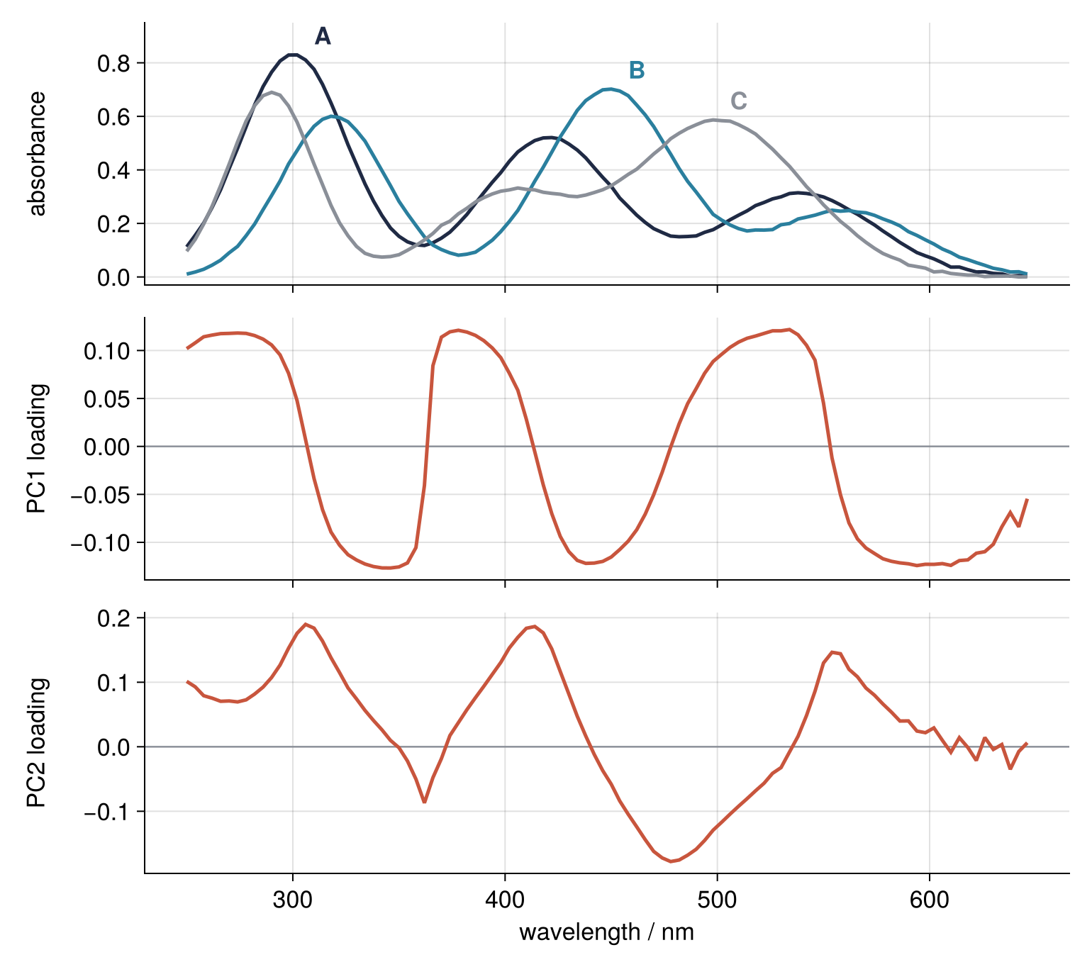
Top: mean absorption spectrum of compounds A, B, and C against wavelength in nm. Middle: PC1 loading, flat plateaus near -0.12 where B absorbs more than C and near +0.12 where C does. Bottom: PC2 loading, peaks near 306 and 414 nm, the bands of A, and a trough near 478 nm.

PC1 looks nothing like a band: level plateaus of −0.11 to −0.13 where B absorbs more than C (338, 450, 622 nm), near +0.12 where C does (270, 378, 526 nm). A high score puts a sample, on balance, above the mean where its loading is positive and below it where negative, so a high PC1 score means C-like, a low one B-like. PC2 reaches +0.19 at 306 and 414 nm, A's strong bands, and −0.18 at 478 nm, where B and C absorb far more than A. It dips below zero, so it is not A's spectrum; pure spectra need a method for non-negative parts, such as NMF or MCR-ALS.

Standardizing makes the plateaus. With every row of Z at standard deviation 1, size buys a wavelength nothing; its weight is set by its correlation with the PC1 scores, and every wavelength where B and C differ well above the noise correlates about equally. For standardized data loadings(M) returns these correlations r. Compare 450 and 622 nm, and the centered fit:

L = loadings(M)
for w in [450, 622]
    j = findfirst(==(w), wavelength)
    @printf("%d nm: r = %+.3f, loadings(M) %+.3f, projection(M) %+.3f   centered only %+.3f\n",
            w, cor(Z[j, :], S[1, :]), L[j, 1], P[j, 1], projection(Mc)[j, 1])
end
difference = means["B"] .- means["C"]
@printf("centered-only PC1 loading against mean B minus mean C: r = %+.2f\n", cor(projection(Mc)[:, 1], difference))

450 nm: r = -0.890, loadings(M) -0.890, projection(M) -0.115   centered only -0.167
622 nm: r = -0.859, loadings(M) -0.859, projection(M) -0.111   centered only -0.020
centered-only PC1 loading against mean B minus mean C: r = -0.99

B minus C is 0.36 at 450 nm and 0.05 at 622 nm, yet r is −0.89 and −0.86, as in loadings(M). A standardized loading marks where the samples differ consistently, not by how much. Centered only, 622 nm falls to an eighth of 450 nm, and the PC1 loading traces mean B minus mean C (r = −0.99): the band shapes, silent where nothing absorbs. A mirrored sign is harmless: flip a column of projection(M) and its scores flip with it.

Scores and both loadings, side by side, make the final figure:

fig = Figure(size = (880, 462))
ax_s = Axis(fig[1:2, 1], xlabel = score_label(1), ylabel = score_label(2))
for (name, color) in COMPOUNDS
    s = compound .== name
    scatter!(ax_s, S[1, s], S[2, s], color = color, markersize = 12)
    text!(ax_s, mean(S[1, s]), maximum(S[2, s]) + 0.8, text = name, color = color, align = (:center, :bottom), font = :bold)
end
ax_top = Axis(fig[1, 2], ylabel = "PC1 loading", yticklabelspace = 52.0)
ax_bot = Axis(fig[2, 2], ylabel = "PC2 loading", xlabel = "wavelength / nm", yticklabelspace = 52.0)
for (i, ax) in enumerate([ax_top, ax_bot])
    hlines!(ax, [0], color = MUTED, linewidth = 1.2)
    lines!(ax, wavelength, P[:, i], color = ACCENT)
end
linkxaxes!(ax_top, ax_bot)
hidexdecorations!(ax_top, grid = false, ticks = false)
colsize!(fig.layout, 1, Auto(1))
colsize!(fig.layout, 2, Auto(1.15))
fig

Left: PC2 score against PC1 score, three separate clusters, B on the left, C on the right, A above. Right: PC1 loading against wavelength in nm, flat plateaus switching between about -0.12 and +0.12, and PC2 loading with peaks near 306 and 414 nm and a trough near 478 nm.

Pitfalls

Passing samples as rows. A table from a CSV file usually has one row per sample. Hand it to fit as it is and MultivariateStats takes the 100 wavelengths for samples and the 60 spectra for variables, without a word:

Mt = fit(PCA, permutedims(Z); maxoutdim = 2)
println("projection: ", size(projection(Mt)), "   scores: ", size(predict(Mt, permutedims(Z))))

projection: (60, 2)   scores: (2, 100)

The "scores plot" from this fit has 100 dots, one per wavelength, and the "loadings" one weight per spectrum. Nothing errors, because both shapes are legal. The same slip in Step 2, dims = 1, standardizes each spectrum instead of each wavelength, as silently. Check the shapes: size(X) is (number of variables, number of samples), size(M, 1) is the number of variables, and size(S, 2) the number of samples. A table with one row per sample goes in as permutedims(X).

Mixing units without scaling. Append a row of a different kind to the spectra, for instance each sample's mass in mg, fit PCA on the result without the transform, and that row becomes the first component:

mass = 50 .+ 5 .* randn(Xoshiro(SEED + 1), size(X, 2))   # mg, its own generator
X_mass = vcat(X, mass')

raw = fit(PCA, X_mass; pratio = 1.0)
Z_mass = StatsBase.transform(fit(ZScoreTransform, X_mass; dims = 2), X_mass)
scaled = fit(PCA, Z_mass; pratio = 1.0)
@printf("without transform: PC1 %.1f %%, loading on mass %+.3f\n", 100 * principalvars(raw)[1] / var(raw), projection(raw)[end, 1])
println("with transform:    PC1 to PC3 ", round.(100 .* principalvars(scaled)[1:3] ./ var(scaled); digits = 1), " %")
@printf("variance of the mass row %.1f mg², of all 100 wavelengths together %.2f\n", var(mass), sum(var(X; dims = 2)))

without transform: PC1 93.7 %, loading on mass -1.000
with transform:    PC1 to PC3 [58.9, 25.1, 6.2] %
variance of the mass row 24.0 mg², of all 100 wavelengths together 1.62

PC1 takes 93.7 % of the variance, loads −1.000 on the mass, and leaves the 100 wavelengths with nothing. Variance comes in the square of the unit, and 24.0 mg² of mass variance swamps the 1.62 of all absorbances together. Standardize first, as Step 2 asks for mixed units, and the shares are back at 58.9, 25.1, and 6.2 %. fit(PCA, ...) removes the means on its own and stores them in mean(M), so centering cannot be forgotten. Scaling can.

Taking the largest variance for the interesting one. PCA orders directions by variance and knows nothing of your labels, and the biggest source of variation is not always the one you are after. Increase the spread of the concentration between samples from 8 % to 35 %:

X35, compound35, conc35 = make_spectra(conc_sd = 0.35)
Z35 = StatsBase.transform(fit(ZScoreTransform, X35; dims = 2), X35)
M35 = fit(PCA, Z35; pratio = 1.0)
S35 = predict(M35, Z35)
println("shares / %: ", round.(100 .* principalvars(M35)[1:3] ./ var(M35); digits = 1),
        @sprintf("   PC1 against concentration r = %+.2f", cor(S35[1, :], conc35)))
println("     sd of PC1 within compound    PC2 at 35 %")
println("        at 8 %      at 35 %")
for (name, _) in COMPOUNDS
    s8, s35 = compound .== name, compound35 .== name
    @printf("  %s    %5.2f       %5.2f      %+5.1f ± %.1f\n", name, std(S[1, s8]), std(S35[1, s35]), mean(S35[2, s35]), std(S35[2, s35]))
end

shares / %: [51.1, 32.5, 11.7]   PC1 against concentration r = -0.97
     sd of PC1 within compound    PC2 at 35 %
        at 8 %      at 35 %
  A     0.95        5.86       -2.2 ± 2.5
  B     1.24        9.63       +7.1 ± 0.6
  C     0.59        4.13       -4.9 ± 3.3

Now PC1 is the concentration (r = −0.97; its sign means nothing), and the first two components hold 51.1 % and 32.5 %. Within a single compound the PC1 scores used to spread by 0.59 to 1.24 and now spread by 4.13 to 9.63, so on PC1 the three compounds overlap completely. Only PC2 still sorts them, B cleanly and A from C partly, since C spreads by 3.3 along it. Look past the first two components, take out a known nuisance before fitting (the first Variation), and if the labels are the goal, train a supervised classifier as in Classification with MLJ.jl.

Variations

Normalize spectra first. Divide each column of X by its sum before the transform, X ./ sum(X; dims = 1), to remove the concentration, and PC3, 6.3 % here, sinks close to the noise floor.
Rebuild the spectra without the noise. With maxoutdim = 3, reconstruct(M, predict(M, Z)) assembles each spectrum from three components alone and leaves the noise floor out; StatsBase.reconstruct(dt, ...) converts it back to absorbance.
Use the labels. fit(MulticlassLDA, Z, compound) from the same package finds the directions that best separate known groups, two for three compounds.
PCA inside an MLJ pipeline. Standardizer() |> PCA(), with the PCA model from MLJMultivariateStatsInterface, holds scaling and PCA in one object, so no new sample gets one without the other; pipelines are in Classification with MLJ.jl.

Cheat sheet

dt = fit(ZScoreTransform, X; dims = 2)       # X: rows variables, columns samples; skip for same-unit spectra
Z = StatsBase.transform(dt, X)               # MultivariateStats has its own transform: qualify it
M = fit(PCA, Z; maxoutdim = 3)               # or pratio = 0.95; default pratio = 0.99; centers, never scales
principalvars(M) ./ var(M)                   # share of each component; cumsum for the running total
S = predict(M, Z)                            # scores: (n_components, n_samples); a single spectrum as a vector
projection(M)                                # loadings: one column per component, unit length, sign arbitrary
loadings(M)                                  # the same, scaled by sqrt(principalvars): correlations if Z is standardized
S_new = predict(M, StatsBase.transform(dt, X_new))   # new samples through the fitted dt and M, never a refit
Z_back = reconstruct(M, S)                   # back from the kept components; StatsBase.reconstruct(dt, Z_back) to units