Compact finite differences: four points per wavelength instead of 26
Afterwards you can read a modified wavenumber plot, explain why compact finite differences resolve short waves with few points, and apply one with findiff.
- Topic
- Numerical calculus
- Field
- Engineering, Physics
- Prerequisites
- Finite differences: the heat equation as a matrix, and why the time step has a limit, The Fourier transform: asking a signal how much of each frequency it contains
- Libraries
findiff 0.13.1matplotlib 3.11.2numpy 2.4.3scipy 1.18.1
py-compact-finite-differences.ipynb, executed with the versions above. The download needs a free account
Run it yourself. In a terminal, this installs exactly the versions above:
pip install numpy==2.4.3 scipy==1.18.1 findiff==0.13.1 matplotlib==3.11.2 jupyterlabThe question
An aeroacoustics code holds the pressure of a sound wave on a grid with points 1 cm apart, and at every time step it needs the gradient \(\partial p/\partial x\), because that is what accelerates the air: \(\rho\,\partial u/\partial t = -\partial p/\partial x\). Send a tone burst of 8.6 kHz down a duct. In air its wavelength is 4 cm, so the grid has four points per wavelength. Here is the burst, and its gradient by the three-point central difference, \(f'_i \approx (f_{i+1} - f_{i-1})/(2h)\), against the exact one; wider formulas and compact finite differences follow in the numbers under the figure.
Show code
import numpy as np
import matplotlib.pyplot as plt

plt.rcParams.update({
    "figure.figsize": (8, 4.4), "figure.dpi": 110,
    "axes.spines.top": False, "axes.spines.right": False,
    "axes.grid": True, "grid.alpha": 0.25,
    "font.size": 11, "lines.linewidth": 1.8,
})
INK, ACCENT, SECOND, MUTED = "#1f2a44", "#c8553d", "#2a7f9e", "#8a8f98"

# a periodic duct of 2.56 m in air; the burst is generated, there is no data
h, N, c_air = 0.01, 256, 343.0              # m, points, m/s
x = np.arange(N) * h
lam0, sigma, x0 = 0.04, 0.08, 1.28          # carrier wavelength, envelope width, center / m
k0 = 2 * np.pi / lam0


def burst(x):
    u = x - x0
    return np.exp(-u**2 / (2 * sigma**2)) * np.cos(k0 * u)


def burst_gradient(x):
    u = x - x0
    return np.exp(-u**2 / (2 * sigma**2)) * (-u / sigma**2 * np.cos(k0 * u) - k0 * np.sin(k0 * u))


def shift(n, j):
    """(shift(n, j) @ f)[i] = f[i + j] on a periodic grid of n points."""
    return np.roll(np.eye(n), j, axis=1)


# central formulas f'_i = sum_j a_j (f_{i+j} - f_{i-j}) / (2h)
EXPLICIT = {"three-point": [1], "five-point": [4 / 3, -1 / 6], "seven-point": [3 / 2, -3 / 10, 1 / 30]}
ALPHA, A6, B6 = 1 / 3, 14 / 9, 1 / 9        # Lele's sixth-order tridiagonal scheme
# one color and opacity per scheme in every figure: the explicit family in SECOND, paler = wider
STYLE = {"three-point": (SECOND, 1.0), "five-point": (SECOND, 0.7), "seven-point": (SECOND, 0.45),
         "compact": (ACCENT, 1.0)}


def explicit(f, a):
    return sum(aj * (np.roll(f, -j) - np.roll(f, j)) for j, aj in enumerate(a, start=1)) / (2 * h)


def compact(f):
    """Solve L f' = R f with a dense solve: transparent, and instant for a few hundred points."""
    n = f.size
    L = np.eye(n) + ALPHA * (shift(n, 1) + shift(n, -1))
    R = A6 * (shift(n, 1) - shift(n, -1)) / (2 * h) + B6 * (shift(n, 2) - shift(n, -2)) / (4 * h)
    return np.linalg.solve(L, R @ f)


p, dp = burst(x), burst_gradient(x)
peak = np.abs(dp).max()
gradients = {name: explicit(p, a) for name, a in EXPLICIT.items()}
gradients["compact"] = compact(p)
print(f"carrier: {c_air / lam0 / 1e3:.2f} kHz, {lam0 / h:.0f} points per wavelength")
for name, g in gradients.items():
    print(f"{name:12s} peak / exact peak = {np.abs(g).max() / peak:.3f}")

near = np.abs(x - x0) <= 0.25
xf = np.linspace(x0 - 0.25, x0 + 0.25, 2001)
fig, (ax0, ax1) = plt.subplots(2, 1, sharex=True)
ax0.plot(100 * (xf - x0), burst(xf), color=INK, lw=1)
ax0.plot(100 * (x[near] - x0), p[near], "o", color=INK, ms=3)
ax0.set(ylabel="p / peak")
ax1.plot(100 * (xf - x0), burst_gradient(xf) / peak, color=INK, lw=1.2)
g3 = gradients["three-point"]
ax1.plot(100 * (x[near] - x0), g3[near] / peak, "o-", color=SECOND, ms=3, lw=0.8)
ax1.text(0.99, 0.95, f"three-point: {100 * np.abs(g3).max() / peak:.0f} % of the peak", transform=ax1.transAxes,
         ha="right", va="top", color=SECOND)
ax1.set(xlabel="x − x₀ / cm", ylabel="∂p/∂x / exact peak", xlim=(-25, 25))
plt.show()
carrier: 8.57 kHz, 4 points per wavelength
three-point  peak / exact peak = 0.632
five-point   peak / exact peak = 0.842
seven-point  peak / exact peak = 0.928
compact      peak / exact peak = 0.989
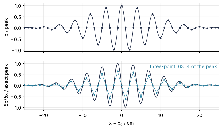
The three-point gradient has the right shape and the wrong size: its peak is 63 % of the true one. Every gradient of a wave this short comes out too small, so a code built on it accelerates the air too little. Widening the stencil, the set of neighbors a formula reads, helps, slowly. The five-point formula reaches 84 % and the seven-point one 93 %. They come from matching Taylor terms over more neighbors, as the three-point formula does, and their coefficients follow in the Formalization.
A compact scheme touches only five function values, like the five-point formula, and gets 98.9 %. It does not compute each derivative on its own: it solves for all of them at once, each tied to its two neighbors. Why does coupling the unknowns buy that much, what does it cost, and where does it stop paying?
The idea: a difference shrinks a wave, it does not bend it
Apply the three-point formula \((f_{i+1} - f_{i-1})/(2h)\) to one sine, \(f = \sin kx\). The identity \(\sin k(x+h) - \sin k(x-h) = 2\sin kh\,\cos kx\) turns it into \(k\cos kx\) times \(\sin(kh)/kh\): the exact derivative, multiplied at every grid point by the same factor, which depends only on \(kh\).
This is not luck of the three-point formula. Shifting \(e^{ikx}\) by one grid point multiplies it by the number \(e^{ikh}\), so any linear rule that is the same at every point, however many neighbors it uses and whether or not it couples them, returns \(e^{ikx}\) times one number. For a centered rule, with opposite weights on opposite sides, that number is \(ik'\) with \(k'\) real: the exact derivative \(ik\,e^{ikx}\) with \(k\) replaced by \(k'\). The factor is \(k'/k\), and each scheme is therefore one curve, its factor against the number of points per wavelength. Here it is at three resolutions, for the three-point formula and for a compact scheme defined in the next section, where its factor is computed:
Show code
n_sine = 48                                   # 48 cm holds a whole number of each wavelength
xs = np.arange(n_sine) * h
fig, axes = plt.subplots(3, 1, figsize=(8, 6.0), sharex=True)
for ax, ppw in zip(axes, [16, 6, 4]):
    k = 2 * np.pi / (ppw * h)
    f, exact = np.sin(k * xs), k * np.cos(k * xs)
    d3, dc = explicit(f, [1]), compact(f)
    use = np.abs(exact) > 0.2 * k                 # where the ratio is not 0 / 0
    r3, rc = d3[use] / exact[use], dc[use] / exact[use]
    spread = max(np.ptp(r3), np.ptp(rc))
    print(f"{ppw:2d} points per wavelength: three-point x {r3.mean():.3f}, compact x {rc.mean():.4f}, "
          f"spread along the grid {spread:.0e}")
    xf = np.linspace(0, 0.16, 801)
    ax.plot(100 * xf, np.cos(k * xf), color=INK, lw=1.2)
    show = xs <= 0.16
    ax.plot(100 * xs[show], d3[show] / k, "o-", color=SECOND, ms=4, lw=0.8)
    ax.plot(100 * xs[show], dc[show] / k, "o", color=ACCENT, ms=4)
    ax.text(0.0, 1.03, f"{ppw} points per wavelength", transform=ax.transAxes, ha="left", va="bottom")
    ax.text(0.73, 1.03, f"three-point × {r3.mean():.3f}", transform=ax.transAxes, ha="right", va="bottom",
            color=SECOND)
    ax.text(1.0, 1.03, f"compact × {rc.mean():.4f}", transform=ax.transAxes, ha="right", va="bottom", color=ACCENT)
    ax.set(ylim=(-1.25, 1.25), ylabel="f′ / k")
axes[-1].set(xlabel="x / cm", xlim=(0, 16))
plt.show()
16 points per wavelength: three-point x 0.974, compact x 1.0000, spread along the grid 1e-14
 6 points per wavelength: three-point x 0.827, compact x 0.9993, spread along the grid 3e-14
 4 points per wavelength: three-point x 0.637, compact x 0.9903, spread along the grid 3e-15
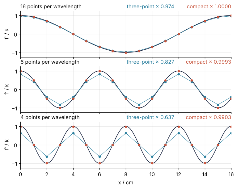
At 16 points per wavelength the three-point factor is 0.974, at 6 it is 0.827, and at 4 it is 0.637, which is the 63 % of the burst. The compact factors are 1.0000, 0.9993, and 0.9903 at the same resolutions. Along each grid the ratio to the exact derivative does not vary beyond round-off, and the dots sit at the right phase: on a single snapshot, a centered scheme gets the amplitude wrong and the phase right. Phase errors appear only once the wave moves.
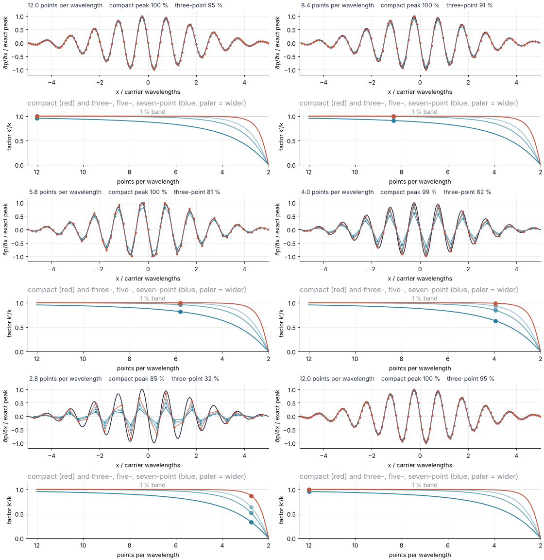
Now let the burst itself get shorter. Below, its points per wavelength fall from 12 to 2.5 while the picture keeps the burst at one size, and the factor of each scheme slides along its curve:
Show code
"""The gradient of a tone burst as the grid thins from 12 to 2.5 points per wavelength.

Renders ../../assets/packet-sweep.gif for the compact finite differences Concept tutorial
(py-compact-finite-differences). Top: the burst's gradient, exact and by four central schemes,
against x in carrier wavelengths, so the burst keeps its size on screen. Bottom: each scheme's
factor k'/k against points per wavelength, with a dot at the burst's carrier. Run it from any directory:

    python scene.py
"""
from pathlib import Path

import numpy as np
import matplotlib.pyplot as plt
from matplotlib.animation import FuncAnimation, PillowWriter

OUT = Path(__file__).resolve().parents[2] / "assets" / "packet-sweep.gif"
INK, ACCENT, SECOND, MUTED = "#1f2a44", "#c8553d", "#2a7f9e", "#8a8f98"
plt.rcParams.update({"axes.spines.top": False, "axes.spines.right": False,
                     "axes.grid": True, "grid.alpha": 0.25, "font.size": 11})

# ---- the schemes of the tutorial: explicit f'_i = sum_j a_j (f_{i+j} - f_{i-j}) / 2h, and Lele's compact one
EXPLICIT = {"three-point": [1], "five-point": [4 / 3, -1 / 6], "seven-point": [3 / 2, -3 / 10, 1 / 30]}
ALPHA, A6, B6 = 1 / 3, 14 / 9, 1 / 9
STYLE = {"three-point": (SECOND, 1.0), "five-point": (SECOND, 0.7), "seven-point": (SECOND, 0.45),
         "compact": (ACCENT, 1.0)}


def factor(name, theta):
    """k'/k at kh = theta."""
    if name == "compact":
        kh = (A6 * np.sin(theta) + B6 / 2 * np.sin(2 * theta)) / (1 + 2 * ALPHA * np.cos(theta))
    else:
        kh = sum(a * np.sin(j * theta) for j, a in enumerate(EXPLICIT[name], start=1))
    return kh / theta


# ---- the burst on a periodic grid with h = 1; its carrier wavelength is ppw grid spacings
N = 512
n_grid = np.arange(N)
I = np.eye(N)
S = {j: np.roll(I, j, axis=1) for j in (-2, -1, 1, 2)}               # (S[j] @ f)[i] = f[i + j]
L = I + ALPHA * (S[1] + S[-1])
R = A6 * (S[1] - S[-1]) / 2 + B6 * (S[2] - S[-2]) / 4
L_inv_R = np.linalg.solve(L, R)                                       # once; every frame reuses it


def gradients(ppw):
    """x in wavelengths, and the exact and four numerical gradients normalized by the exact peak."""
    k, sigma, x0 = 2 * np.pi / ppw, 2 * ppw, N / 2                  # envelope of two wavelengths, as in the tutorial
    u = n_grid - x0
    env = np.exp(-u**2 / (2 * sigma**2))
    f = env * np.cos(k * u)
    exact = env * (-u / sigma**2 * np.cos(k * u) - k * np.sin(k * u))
    out = {name: sum(a * (np.roll(f, -j) - np.roll(f, j)) for j, a in enumerate(c, start=1)) / 2
           for name, c in EXPLICIT.items()}
    out["compact"] = L_inv_R @ f
    peak = np.abs(exact).max()
    return u / ppw, {name: g / peak for name, g in out.items()}


def exact_fine(ppw, xi):
    """The exact gradient on a fine grid of xi, in wavelengths, normalized like gradients()."""
    sigma_w = 2.0
    env = np.exp(-xi**2 / (2 * sigma_w**2))
    g = env * (-xi / sigma_w**2 * np.cos(2 * np.pi * xi) - 2 * np.pi * np.sin(2 * np.pi * xi))
    return g / np.abs(g).max()


# ---- frame schedule: hold, sweep 12 -> 2.5 points per wavelength, hold, sweep back fast
sweep = np.geomspace(12, 2.5, 66)
schedule = [12.0] * 6 + list(sweep) + [2.5] * 10 + list(sweep[-6::-6])

# ---- figure, drawn once
fig, (ax0, ax1) = plt.subplots(2, 1, figsize=(7.0, 4.8), dpi=80, layout="constrained",
                               height_ratios=[1.15, 1])            # 560 x 384 px
xi = np.linspace(-5, 5, 1001)
ax0.plot(xi, exact_fine(12, xi), color=INK, lw=1.4)
lines = {}
for name, (color, alpha) in STYLE.items():
    (lines[name],) = ax0.plot([], [], "o-", color=color, alpha=alpha, ms=2.5, lw=1.0)
ax0.set(xlim=(-5, 5), ylim=(-1.2, 1.2), xlabel="x / carrier wavelengths", ylabel="∂p/∂x / exact peak")
title = ax0.set_title("", loc="left", fontsize=11, color=INK)

ppw_axis = np.geomspace(12, 2.0, 400)
ax1.fill_between(ppw_axis, 0.99, 1.0, color=MUTED, alpha=0.30, lw=0)
dots = {}
for name, (color, alpha) in STYLE.items():
    ax1.plot(ppw_axis, factor(name, 2 * np.pi / ppw_axis), color=color, alpha=alpha, lw=1.6)
    (dots[name],) = ax1.plot([], [], "o", color=color, alpha=alpha, ms=7)
ax1.text(7.0, 1.015, "1 % band", color=MUTED, va="bottom", ha="center")
ax1.set(xlim=(12.4, 2.0), ylim=(0, 1.15), xlabel="points per wavelength", ylabel="factor k′/k")
ax1.set_title("compact (red) and three-, five-, seven-point (blue, paler = wider)", loc="left",
              color=MUTED)


def update(i):
    ppw = schedule[i]
    xw, g = gradients(ppw)
    view = np.abs(xw) <= 5
    for name in STYLE:
        lines[name].set_data(xw[view], g[name][view])
        dots[name].set_data([ppw], [factor(name, 2 * np.pi / ppw)])
    title.set_text(f"{ppw:4.1f} points per wavelength    compact peak {100 * np.abs(g['compact']).max():.0f} %"
                   f"    three-point {100 * np.abs(g['three-point']).max():.0f} %")


OUT.parent.mkdir(exist_ok=True)
FuncAnimation(fig, update, frames=len(schedule)).save(OUT, writer=PillowWriter(fps=12))
plt.close(fig)
print(f"{len(schedule)} frames, {OUT.stat().st_size / 1e6:.2f} MB")
In a simulation the factor turns into a speed. A code that steps the wave equation with this derivative replaces \(\partial/\partial x\), which acts on \(e^{ikx}\) as \(ik\), by \(ik'\), so the frequency becomes \(\omega = ck'\) instead of \(ck\) and a wave of wavenumber \(k\) moves at \(\omega/k = c\,k'/k\). Short waves fall behind the long ones and a burst smears into a trail of ripples. The wave equation with leapfrog finite differences shows the same effect coming from the time step. With the three-point factor of 0.637, the 8.6 kHz tone would cross the duct at 64 % of the speed of sound.
Coupling the derivatives: a wide stencil in a small one
Lele's scheme, published in 1992, ties each unknown derivative to its two neighbors' derivatives with weight 1/3, and puts a five-point combination of function values on the other side:
No derivative can be computed alone, so all \(N\) of them are the unknowns of one tridiagonal system, \(L\,f' = R\,f\), with \(L\) the left side and \(R\) the right side as matrices. The factor promised in the previous section takes one line. Put \(f = e^{ikx}\) in, write \(f' = ik'\,e^{ikx}\) and \(\theta = kh\); the left side becomes \((1 + \tfrac{2}{3}\cos\theta)\,ik'e^{ikx_i}\) and the right side \(i\,(\tfrac{14}{9}\sin\theta + \tfrac{1}{18}\sin 2\theta)\,e^{ikx_i}/h\), so
the curve already drawn in red. Dividing by \(1 + \tfrac{2}{3}\cos\theta\) is what lifts it: the denominator is smallest for short waves, where the numerator falls short the most.
Solving the system is the same as multiplying \(f\) by \(L^{-1}R\), and that matrix is a stencil too. Here is one of its rows, for 64 points:
Show code
n64 = 64
L64 = np.eye(n64) + ALPHA * (shift(n64, 1) + shift(n64, -1))
R64 = A6 * (shift(n64, 1) - shift(n64, -1)) / 2 + B6 * (shift(n64, 2) - shift(n64, -2)) / 4   # h = 1
M = np.linalg.solve(L64, R64)
i0 = n64 // 2
row = M[i0]
w7 = np.array(EXPLICIT["seven-point"]) / 2
print("offset            " + "".join(f"{j:9d}" for j in range(1, 7)))
print("compact, L^-1 R   " + "".join(f"{row[i0 + j]:+9.3f}" for j in range(1, 7)))
print("seven-point       " + "".join(f"{w:+9.4f}" for w in w7) + "        0" * 3)
print("successive ratio  " + "".join(f"{row[i0 + j + 1] / row[i0 + j]:+9.3f}" for j in range(1, 7)))

offsets = np.arange(-8, 9)
fig, ax = plt.subplots(figsize=(7, 3.2))
ax.axhline(0, color=MUTED, lw=1)
ax.plot(offsets, row[i0 + offsets], "o", color=ACCENT, ms=6)
w7_full = np.concatenate([-w7[::-1], [0], w7])
c7, a7 = STYLE["seven-point"]
ax.plot(np.arange(-3, 4), w7_full, "s", color=c7, alpha=a7, ms=6, mfc="none", mew=1.8)
ax.text(1.35, row[i0 + 1], "compact, L⁻¹R", color=ACCENT, va="center")
ax.text(-1.35, w7[0] * -1, "seven-point", color=c7, alpha=max(a7, 0.7), ha="right", va="center")
ax.set(xlabel="offset from the point j", ylabel="weight × h", xlim=(-8.5, 8.5))
plt.show()
offset                    1        2        3        4        5        6
compact, L^-1 R      +0.879   -0.304   +0.116   -0.044   +0.017   -0.006
seven-point         +0.7500  -0.1500  +0.0167        0        0        0
successive ratio     -0.346   -0.382   -0.382   -0.382   -0.382   -0.382
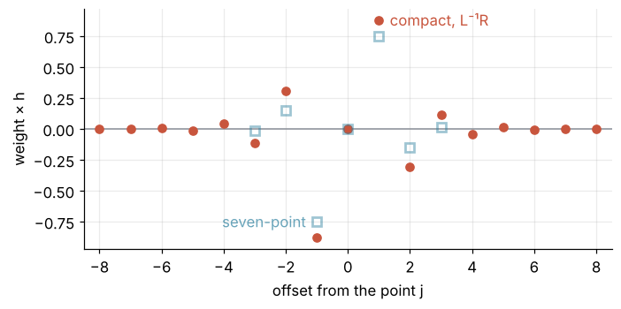
The seven-point formula has weights 0.750, −0.150, and 0.0167 at offsets 1 to 3 and nothing beyond. The compact row starts at 0.879, −0.304, 0.116, and keeps going: −0.044, 0.017, −0.006, and from offset 3 on each weight is −0.382 times the one before, all the way around the grid. Beyond offset 2 the right side of Lele's equation is silent, so the weights obey the left side alone, \(w_{j-1}/3 + w_j + w_{j+1}/3 = 0\). Trying \(w_j = z^j\) turns that into \(z^2 + 3z + 1 = 0\), whose root \(-0.382\) is the decay per offset. The coupling buys an infinitely wide stencil with geometrically decaying weights, while the code stores three diagonals and touches five function values. That is where the extra resolution comes from.
Free account
The second half of this tutorial needs a free account
Sign in, or create an account with your email address, and the page goes on right here. The account costs nothing and also brings the notebook download, collections, and done marks.
Still to come
- Formalization
- See it in code
- Where it shows up
- Further reading