The wave equation with leapfrog finite differences: a pulse on a string (Python)

The problem: does a pulse on a string come back as it left?

A string 1 m long is clamped at both ends. You lift a Gaussian bump 3 cm wide at x = 0.3 m and let go. The wave equation

\[\frac{\partial^2 u}{\partial t^2} = c^2\,\frac{\partial^2 u}{\partial x^2},\]

with \(u\) the displacement and wave speed c = 1 m/s, says what happens next: the bump splits into two halves that run apart, flip over at the clamped ends, and meet again.

After one round trip, 2L/c = 2 s for the length L = 1 m, the string has exactly its starting shape. That is a sharp test for the leapfrog scheme, the finite difference method that replaces both second derivatives by differences on a grid and moves the whole string forward with one line of NumPy per step. Its only parameter is the Courant number C = cΔt/Δx, the distance the wave travels in one time step, counted in grid spacings.

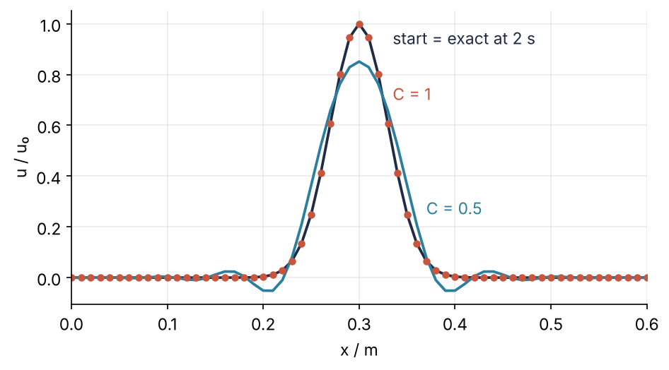
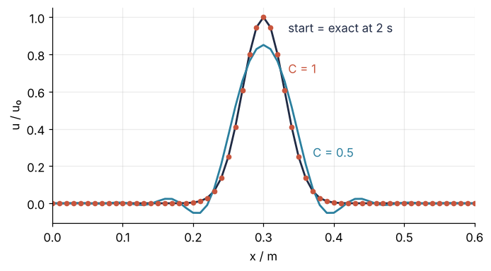
String displacement u / u0 against x in m after a 2 s round trip. C = 1 dots sit on the starting shape; the C = 0.5 curve returns at 0.85 of the height, wider, with dips on both sides.

At C = 1 the computed string comes back to within 2 × 10⁻¹⁵, the rounding level of the arithmetic. At C = 0.5, with twice as many steps, it comes back at 85 % of its height, wider, with dips on both sides. Step 6 draws this figure from the runs of the steps before it. At C = 1.01 there is no pulse left to draw: the error grows by a third every step and passes the height of the pulse before the round trip is over.

Setup

NumPy does the arithmetic and Matplotlib the figures. The constants are the string and the pulse from the problem.

import numpy as np
import matplotlib.pyplot as plt

L = 1.0        # string length, m
c = 1.0        # wave speed, m/s
x0 = 0.3       # pulse center, m
sigma = 0.03   # pulse width, m

plt.rcParams.update({                      # the look of every figure below
    "figure.figsize": (7, 3.6), "figure.dpi": 110,
    "axes.spines.top": False, "axes.spines.right": False,
    "axes.grid": True, "grid.alpha": 0.25,
    "font.size": 11, "lines.linewidth": 1.8,
})
INK, ACCENT, SECOND, MUTED = "#1f2a44", "#c8553d", "#2a7f9e", "#8a8f98"

print(f"round trip 2L/c = {2 * L / c:.1f} s")

round trip 2L/c = 2.0 s

Step 1: Put the string on a grid and lay down the pulse

A hundred intervals of 1 cm, so 101 points with both ends included. The pulse is a function of x, because later steps need it on other grids and at shifted positions:

N = 100
x = np.linspace(0, L, N + 1)
dx = x[1] - x[0]

def pulse(x):
    return np.exp(-(x - x0)**2 / (2 * sigma**2))

u0 = pulse(x)
print(f"dx = {dx:.2f} m, {sigma / dx:.0f} points per sigma")
print(f"pulse at the ends before clamping: {u0[0]:.1e}, {u0[-1]:.1e}")
u0[[0, -1]] = 0.0                          # the clamped ends

dx = 0.01 m, 3 points per sigma
pulse at the ends before clamping: 1.9e-22, 6.0e-119

Setting the ends to zero changes the pulse by 1.9 × 10⁻²², so the clamp costs nothing measurable here. Three points per σ is deliberately coarse. It resolves the bump, barely, and Step 5 shows what that costs.

Step 2: Replace both second derivatives by differences

The second derivative at a grid point is, to second order in the spacing, the two neighbors minus twice the point, divided by the spacing squared. Write \(u_j^n\) for the displacement at point j and time level n, and \(\delta^2 u_j = u_{j+1} - 2u_j + u_{j-1}\) for that second difference. Doing the same in time and in space turns the wave equation into

\[\frac{u_j^{n+1} - 2u_j^n + u_j^{n-1}}{\Delta t^2} = c^2\,\frac{\delta^2 u_j^n}{\Delta x^2} \quad\Longrightarrow\quad u_j^{n+1} = 2u_j^n - u_j^{n-1} + C^2\,\delta^2 u_j^n ,\]

and of c, Δt, and Δx only the Courant number C is left. Step 4 also needs the forward difference \(\delta_+ u_j = u_{j+1} - u_j\), Δx times the slope between two neighbors. On the interior points u[2:], u[1:-1], and u[:-2] are \(u_{j+1}\), \(u_j\), and \(u_{j-1}\), the array shifted by one point each way, so the update is one slice expression. A single spike shows the weights it hands out:

def leapfrog(u, u_old, C2):
    u_new = np.zeros_like(u)               # the ends stay at zero: this is the clamp
    u_new[1:-1] = 2 * u[1:-1] - u_old[1:-1] + C2 * (u[2:] - 2 * u[1:-1] + u[:-2])
    return u_new

spike = np.zeros(7)
spike[3] = 1.0
for C in [1.0, 0.5]:
    print(f"C = {C}: new values at points 2, 3, 4:", leapfrog(spike, np.zeros(7), C**2)[2:5])

C = 1.0: new values at points 2, 3, 4: [1. 0. 1.]
C = 0.5: new values at points 2, 3, 4: [0.25 1.5  0.25]

The spike sends C², 2 − 2C², C² to its neighbors and itself. At C = 1 the middle weight vanishes: the new value is the sum of the two neighbors minus the old value, and information moves exactly one point per step, as the wave does. The time difference reaches from the old level across the current one to the new, as one frog leaps over another: hence the name.

Step 3: Take the first step from the initial velocity

Leapfrog needs two earlier levels, and the start provides one level and a velocity \(v^0\). A Taylor expansion fills the gap: \(u(\Delta t) = u + \Delta t\,u_t + \tfrac12\Delta t^2 u_{tt}\), and the wave equation turns \(u_{tt}\) into \(c^2 u_{xx}\), so

\[u_j^1 = u_j^0 + \Delta t\, v_j^0 + \tfrac{C^2}{2}\,\delta^2 u_j^0 .\]

The string is released from rest; a different initial velocity goes into v0:

def first_step(u0, v0, dt, C2):
    u1 = np.zeros_like(u0)
    u1[1:-1] = u0[1:-1] + dt * v0[1:-1] + 0.5 * C2 * (u0[2:] - 2 * u0[1:-1] + u0[:-2])
    return u1

dt = dx / c                                # C = 1
u1 = first_step(u0, np.zeros_like(x), dt, 1.0)
u1_exact = 0.5 * (pulse(x - c * dt) + pulse(x + c * dt))
print(f"largest difference from the exact u at t = dt: {np.abs(u1 - u1_exact).max():.1e}")

largest difference from the exact u at t = dt: 4.4e-16

At C = 1 the first step is the average of the shape shifted by one point each way, which is d'Alembert's exact solution at t = Δt (Step 4), here to 4 × 10⁻¹⁶. Starting with u_old = u0 instead looks harmless and is the first pitfall.

Step 4: Run one round trip and check it against the exact solution

The exact solution is d'Alembert's: the shape split into two halves running in opposite directions, \(u = \tfrac12[f(x - ct) + f(x + ct)]\). Clamped ends enter through \(f\). Extend the pulse beyond each wall by an upside-down mirror image, and repeat with period 2L. A pulse and its image always cancel at the wall, so u = 0 there at every time.

run steps the string to t_end and keeps every level. It rounds the step count and recomputes Δt, because t_end / dt is not always whole (C = 0.9 in Step 5), and returns the Courant number it used. It also returns a second check, the scheme's own energy: the kinetic energy between two levels, from \((u^{n+1} - u^n)/\Delta t\), plus \(\tfrac12 c^2 \sum \delta_+u^{n+1}\,\delta_+u^n/\Delta x\), the product of the slopes at both levels. Leapfrog conserves exactly this quantity, up to rounding. The textbook energy at a single level wobbles by 3 % here even though the solution is exact, so it is not the check.

def exact(x, t):
    def f(s):                              # the pulse, odd about both walls, period 2L
        s = np.mod(s, 2 * L)
        return np.where(s <= L, pulse(s), -pulse(2 * L - s))
    return 0.5 * (f(x - c * t) + f(x + c * t))

def energy(u_new, u, dt, dx):
    kinetic = 0.5 * np.sum(((u_new - u) / dt)**2) * dx
    strain = 0.5 * c**2 * np.sum(np.diff(u_new) * np.diff(u)) / dx
    return kinetic + strain

def run(C, N, t_end, v0=None):
    x = np.linspace(0, L, N + 1)
    dx = x[1] - x[0]
    steps = round(t_end / (C * dx / c))
    dt = t_end / steps
    C2 = (c * dt / dx)**2
    u0 = pulse(x)
    u0[[0, -1]] = 0.0
    v0 = np.zeros_like(x) if v0 is None else v0
    U = [u0, first_step(u0, v0, dt, C2)]
    for n in range(steps - 1):
        U.append(leapfrog(U[-1], U[-2], C2))
    U = np.array(U)
    E = np.array([energy(U[n + 1], U[n], dt, dx) for n in range(steps)])
    return x, dt * np.arange(steps + 1), U, np.sqrt(C2), E

x, t, U, C, E = run(1.0, 100, 2.0)
for t_check in [0.5, 2.0]:
    n = round(t_check / t[1])
    print(f"t = {t[n]:.1f} s: largest deviation from exact {np.abs(U[n] - exact(x, t[n])).max():.1e}")
print(f"relative energy drift over the round trip: {np.ptp(E) / E[0]:.1e}")

t = 0.5 s: largest deviation from exact 1.6e-15
t = 2.0 s: largest deviation from exact 2.3e-15
relative energy drift over the round trip: 5.1e-16

Both deviations and the energy drift are at the rounding level: at C = 1 the scheme is exact on the grid points. The levels show how it gets there, shaded from light to dark in time:

fig, ax = plt.subplots()
for t_snap, alpha, (x_lab, y_lab) in zip([0, 0.25, 0.5, 1.0], [0.3, 0.5, 0.75, 1.0],
                                         [(0.345, 0.85), (0.58, 0.5), (0.83, 0.45), (0.73, -0.95)]):
    n = round(t_snap / t[1])
    ax.plot(x, U[n], color=ACCENT, alpha=alpha)
    ax.text(x_lab, y_lab, f"t = {t_snap:g} s", color=ACCENT, alpha=0.55 + 0.45 * alpha)   # labels stay legible
for wall in [0, L]:
    ax.axvline(wall, color=MUTED, lw=1, ls="--")
ax.set(xlabel="x / m", ylabel="u / u₀", ylim=(-1.15, 1.15))
plt.show()

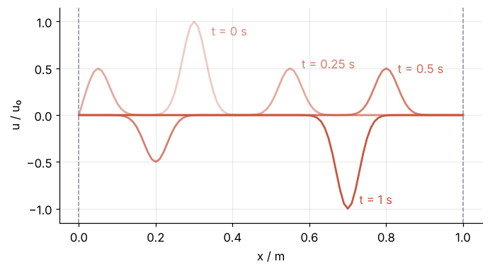
String displacement u / u0 against x in m at t = 0, 0.25, 0.5, and 1 s, leapfrog at C = 1. The pulse splits into two halves, the left half flips at the clamped end x = 0, and at t = 1 s an inverted pulse sits at x = 0.7 m.

The left half reaches the wall at t = 0.3 s and comes back upside down. At t = 1 s both halves, each flipped once, overlap at x = 0.7 m as one inverted pulse, the mirror image of the start.

Step 5: Lower the Courant number and watch the pulse fall apart

An ODE solver such as solve_ivp gets more accurate with smaller steps. Leapfrog on a wave does not:

runs = {}
for C_try in [0.5, 0.9]:
    x, t, U, C, E = run(C_try, 100, 2.0)
    runs[C_try] = (x, U[-1])
    print(f"C = {C:.4f}, {len(t) - 1} steps: peak {U[-1].max():.3f}, lowest {U[-1].min():.3f}, "
          f"deviation {np.abs(U[-1] - exact(x, t[-1])).max():.3f}, energy drift {np.ptp(E) / E[0]:.0e}")

C = 0.5000, 400 steps: peak 0.851, lowest -0.052, deviation 0.149, energy drift 4e-15
C = 0.9009, 222 steps: peak 0.976, lowest -0.000, deviation 0.024, energy drift 1e-15

At C = 0.5 the pulse comes back at 0.851 of its height, with dips to −0.052 and a deviation of 0.149. At C = 0.9 it is 0.024, thirteen orders of magnitude above C = 1. The cause is numerical dispersion. Put a single wave \(u_j^n = e^{i(kj\Delta x - \omega n\Delta t)}\) into the update of Step 2. Each second difference multiplies it by \(-4\sin^2\) of half its phase step, ωΔt in time and kΔx in space, and the square root of what is left is

\[\sin\frac{\omega\Delta t}{2} = C\,\sin\frac{k\Delta x}{2} .\]

At C = 1 this gives ω = ck for every wavelength. Below 1 the phase speed ω/k falls short of c, and more so for short waves:

def speed_ratio(C, points_per_wavelength):
    k_dx = 2 * np.pi / points_per_wavelength
    return 2 * np.arcsin(C * np.sin(k_dx / 2)) / (C * k_dx)

print("points per wavelength:   16      8      6      4")
for C in [1.0, 0.9, 0.5]:
    print(f"C = {C}:          " + "  ".join(f"{speed_ratio(C, p):.3f}" for p in [16, 8, 6, 4]))

points per wavelength:   16      8      6      4
C = 1.0:          1.000  1.000  1.000  1.000
C = 0.9:          0.999  0.995  0.991  0.976
C = 0.5:          0.995  0.981  0.965  0.920

A Gaussian has no single wavelength, but its spectrum falls as \(e^{-k^2\sigma^2/2}\), so waves shorter than about 2σ carry under 1 % of it. Three points per σ is six points across the shortest wave that matters, where C = 0.5 lags by 3.5 %. The rule for your own pulse: count the points across the shortest feature you care about. Refine the grid at C = 0.5:

for N in [50, 100, 200, 400]:
    x, t, U, C, E = run(0.5, N, 2.0)
    n_half = round(0.5 / t[1])
    print(f"N = {N:3d}: {sigma * N / L:4.1f} points per sigma, deviation at 0.5 s "
          f"{np.abs(U[n_half] - exact(x, t[n_half])).max():.4f}, at 2 s {np.abs(U[-1] - exact(x, t[-1])).max():.4f}")

N =  50:  1.5 points per sigma, deviation at 0.5 s 0.1394, at 2 s 0.3831
N = 100:  3.0 points per sigma, deviation at 0.5 s 0.0413, at 2 s 0.1487
N = 200:  6.0 points per sigma, deviation at 0.5 s 0.0101, at 2 s 0.0216
N = 400: 12.0 points per sigma, deviation at 0.5 s 0.0025, at 2 s 0.0016

At 0.5 s the last two halvings of Δx each divide the error by 4, as a second-order scheme promises. At 2 s the last halving divides it by 14, close to 16. A round trip is a full period, so each wave comes back as cos(2π + ε) ≈ 1 − ε²/2, with a phase error ε that shrinks with Δx²: the error is of order ε², so Δx⁴. The energy drift is 4 × 10⁻¹⁵: nothing is lost, only moved into short waves that lag behind. The cure is more points, never a smaller C.

Step 6: Cross the Courant limit and draw the round trip

Push C just past 1. The shortest grid wave, two points per wavelength, has kΔx = π, and Step 5's relation then demands sin(ωΔt/2) = C > 1. No real ω does that. With ωΔt/2 = π/2 + iy the sine becomes cosh y = C, and the wave's amplitude is multiplied by \(e^{2y} = 2C^2 - 1 + 2C\sqrt{C^2 - 1}\) every step instead of oscillating.

The cell runs 200 steps and compares the growth per step with that factor. It also prints the signs of the string near x = 0.3 m, because a wave with two points per wavelength alternates in sign from point to point. x[None, :] and t[:, None] turn the two vectors into a row and a column, so exact fills one row per step in a single call:

x, t, U, C, E = run(1.01, 100, 200 * 1.01 * dx / c)
err = np.abs(U - exact(x[None, :], t[:, None])).max(axis=1)
for n in range(110, 201, 10):
    print(f"step {n}: deviation {err[n]:8.1e}, growth per step {(err[n] / err[n - 10])**0.1:.2f}")
print("signs at x = 0.25 to 0.35 m, step 140:", np.sign(U[140, 25:36]).astype(int))
print(f"growth of the shortest grid wave: {2 * C**2 - 1 + 2 * C * np.sqrt(C**2 - 1):.3f}")

step 110: deviation  2.5e-03, growth per step 0.98
step 120: deviation  5.0e-03, growth per step 1.07
step 130: deviation  5.3e-02, growth per step 1.27
step 140: deviation  8.4e-01, growth per step 1.32
step 150: deviation  1.4e+01, growth per step 1.32
step 160: deviation  2.2e+02, growth per step 1.32
step 170: deviation  3.6e+03, growth per step 1.32
step 180: deviation  5.9e+04, growth per step 1.32
step 190: deviation  9.6e+05, growth per step 1.32
step 200: deviation  1.6e+07, growth per step 1.32
signs at x = 0.25 to 0.35 m, step 140: [-1  1 -1  1 -1  1 -1  1 -1  1 -1]
growth of the shortest grid wave: 1.327

fig, ax = plt.subplots(figsize=(7, 3.4))
ax.semilogy(np.arange(1, len(t)), err[1:], color=SECOND)
ax.axhline(1, color=MUTED, lw=1, ls="--")
ax.text(5, 3, "pulse height", color=MUTED)
ax.text(166, 1e4, "C = 1.01", color=SECOND, ha="right")
ax.set(xlabel="step", ylabel="largest error / u₀", xlim=(0, 200), ylim=(1e-5, 1e8), yticks=[1e-4, 1, 1e4, 1e8])
plt.show()

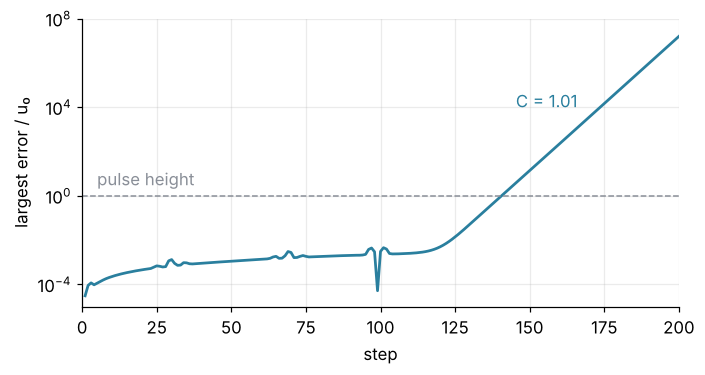
Largest error relative to the pulse height against step number, log scale, for C = 1.01. The error stays below 10⁻² until about step 120, then rises on a straight line and crosses the dashed pulse-height level near step 140.

For 120 steps the error stays below 1 % of the pulse. Then it climbs on a straight line, which on a log scale means the same factor every step, 1.32 measured against 1.327 predicted, and it crosses the pulse height near step 140. The alternating signs say which wave it is.

The Gaussian contains none of that wave; the rounding error supplies it, as Floating-point numbers explains. The same substitution gives the limit of any explicit scheme you write. For the heat equation in py-pde from the ground up Δt shrinks with Δx²; for waves only with Δx.

That leaves the figure from the motivation, the round trips of Steps 4 and 5 against the start:

x1, t1, U1, _, _ = run(1.0, 100, 2.0)
x5, u5 = runs[0.5]
fig, ax = plt.subplots()
ax.plot(x1, U1[0], color=INK)
ax.plot(x5, u5, color=SECOND)
ax.plot(x1, U1[-1], "o", color=ACCENT, ms=4)
ax.text(0.335, 0.92, "start = exact at 2 s", color=INK)
ax.text(0.335, 0.70, "C = 1", color=ACCENT)
ax.text(0.37, 0.25, "C = 0.5", color=SECOND)
ax.set(xlabel="x / m", ylabel="u / u₀", xlim=(0, 0.6))
plt.show()

String displacement u / u0 against x in m after a 2 s round trip. C = 1 dots sit on the starting shape; the C = 0.5 curve returns at 0.85 of the height, wider, with dips on both sides.

Pitfalls

Starting with the shape twice. Setting u_old = u0.copy() and stepping from there is the obvious start, and at C = 1 it even passes the round-trip check. Between periods it does not:

for N in [100, 200, 400]:
    x = np.linspace(0, L, N + 1)
    dt = (x[1] - x[0]) / c                 # C = 1
    u = pulse(x)
    u[[0, -1]] = 0.0
    u_old = u.copy()                       # the shortcut instead of first_step
    levels = [u]
    for n in range(round(2.0 / dt)):
        u, u_old = leapfrog(u, u_old, 1.0), u
        levels.append(u)
    n_half = round(0.5 / dt)
    print(f"N = {N}: deviation at t = 0.5 s {np.abs(levels[n_half] - exact(x, 0.5)).max():.1e}, "
          f"at t = 2 s {np.abs(levels[-1] - exact(x, 2.0)).max():.1e}")

N = 100: deviation at t = 0.5 s 5.2e-02, at t = 2 s 2.0e-15
N = 200: deviation at t = 0.5 s 2.5e-02, at t = 2 s 2.9e-15
N = 400: deviation at t = 0.5 s 1.3e-02, at t = 2 s 2.7e-15

At t = 0.5 s the string is off by 5 % of the amplitude, and the error halves with Δx: first order, from a start that ignores the curvature term of Step 3. At t = 2 s it is gone. At C = 1 every grid wave moves at exactly c (Step 5), so the computed motion repeats after one period, 2L/c, whatever the two starting levels were, and the round trip returns any start as itself. Check at a time that is not a period, as Step 4 does at 0.5 s, and take the first step from Step 3.

Taking dispersion for physics. Ripples behind a pulse look like a stiff string or a dispersive medium, and in a synthetic seismogram like the coda that follows a real arrival. Halve Δx at fixed C. Numerical ripples shrink by a factor of 4 or more (Step 5), physical ones stay.

A time step that was fine on the old grid. You refine from N = 100 to 200 and keep Δt = 0.01 s, and C has become 2: the alternating-sign wave of Step 6 passes 10 at step 16. The same happens when you compute Δt from an average wave speed for a string of two materials or layered rock, where the largest c sets the limit. Compute Δt from C, the current Δx, and the largest c every time you change any of them.

Variations

One-way pulse. Pass v0 = -c * dpulse(x), with dpulse the derivative of the pulse, and the whole bump travels right; first_step takes the velocity unchanged.
A free end. Replace the clamp at x = L by a ghost value one point past the end that mirrors its neighbor, \(u_{N+1} = u_{N-1}\), so that ∂u/∂x = 0 and the update runs at j = N too. The pulse reflects there without flipping and comes back upright after two round trips, 4L/c = 4 s; at C = 1 the deviation is 4 × 10⁻¹⁶.
A string of two materials. Make c an array and C2 one value per point, with the limit set by the largest c. The pulse partly reflects at the joint, as a seismic wave does at a layer boundary.
A membrane. The same update in two dimensions with the five-point Laplacian. The limit becomes C ≤ 1/√2, and no C is free of dispersion in every direction.

Cheat sheet

x = np.linspace(0, L, N + 1); dx = x[1] - x[0]
dt = C * dx / c_max                        # C <= 1, with the largest wave speed
C2 = (c * dt / dx)**2
u_old, u = u0, first_step(u0, v0, dt, C2)  # u0 + dt v0 + C2/2 d2 u0, never u_old = u0
u_new[1:-1] = 2*u[1:-1] - u_old[1:-1] + C2*(u[2:] - 2*u[1:-1] + u[:-2])
u_new[[0, -1]] = 0.0                       # clamped ends
E = 0.5*np.sum(((u_new - u)/dt)**2)*dx + 0.5*c**2*np.sum(np.diff(u_new)*np.diff(u))/dx
# C = 1 is exact in 1D with constant c; below 1, more points per wavelength against dispersion