curve_fit from the ground up: the Michaelis-Menten constants of an enzyme (Python)

The problem: two constants from twelve rates

An enzyme assay gives you twelve numbers: the initial rate \(v\) of the reaction at twelve substrate concentrations \(S\) from 0.5 to 50 mM, each rate with its own error bar. What you want from them is two numbers, the constants of the Michaelis-Menten law

\[v = \frac{V_\mathrm{max}\, S}{K_m + S} .\]

\(V_\mathrm{max}\) is the plateau, the rate of an enzyme saturated with substrate. \(K_m\) is the concentration at which the rate reaches half the plateau, so a small \(K_m\) means an enzyme that works at half speed on little substrate. scipy.optimize.curve_fit gets both constants, with their errors, from one call.

The law is not linear in \(K_m\), so neither a straight-line fit nor np.polyfit can fit it as written. The old way around this is to plot \(1/v\) against \(1/S\), which turns the law into a straight line. The price is that the reciprocal makes the smallest and least certain rates into the largest values, and those end up steering the line. Step 6 measures how far that throws \(K_m\) off on the same data.

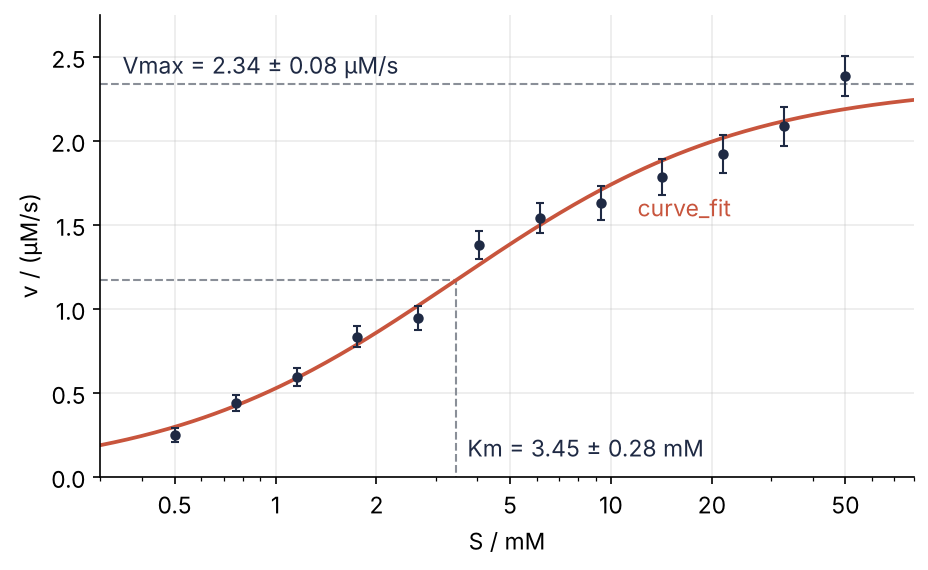
Initial rate in µM/s against substrate concentration in mM on a logarithmic axis. Dots with error bars: twelve measured rates. Line: the curve_fit result, rising to a dashed plateau at Vmax = 2.34 µM/s, with Km = 3.45 mM marked where the curve reaches half the plateau.

This is where we end up: the fitted law follows the twelve rates, levels off at \(V_\mathrm{max} = 2.34 \pm 0.08\) µM/s, and reaches half of that at \(K_m = 3.45 \pm 0.28\) mM. The rest of this tutorial builds the weighted curve_fit call behind it and checks that its answer deserves the ± signs.

Setup

The rates are simulated, so that we know the answer the fit should find: \(V_\mathrm{max} = 2.4\) µM/s and \(K_m = 3.5\) mM. Each rate gets an error of 0.03 µM/s plus 4 % of the rate, and noise drawn from a seeded generator (Random numbers with numpy.random explains default_rng). Replace S, v, and sigma with your own measurements and everything below runs unchanged.

import numpy as np
import matplotlib.pyplot as plt
from scipy.optimize import curve_fit

plt.rcParams.update({
    "figure.figsize": (7, 4), "figure.dpi": 110,
    "axes.spines.top": False, "axes.spines.right": False,
    "axes.grid": True, "grid.alpha": 0.25,
    "font.size": 11, "lines.linewidth": 1.8,
})
INK, ACCENT, SECOND, MUTED = "#1f2a44", "#c8553d", "#2a7f9e", "#8a8f98"

Vmax_true, Km_true = 2.4, 3.5                       # µM/s, mM: what the fit should find
rng = np.random.default_rng(41)
S = np.geomspace(0.5, 50, 12)                       # substrate concentration, mM
v_true = Vmax_true * S / (Km_true + S)
sigma = 0.03 + 0.04 * v_true                        # error of each rate, µM/s
v = v_true + sigma * rng.standard_normal(S.size)    # measured initial rate, µM/s

for name, row in [("S / mM", S), ("v / (µM/s)", v), ("σ / (µM/s)", sigma)]:
    print(f"{name:11s}", " ".join(f"{x:5.2f}" for x in row))

S / mM       0.50  0.76  1.16  1.76  2.67  4.06  6.16  9.37 14.24 21.64 32.90 50.00
v / (µM/s)   0.25  0.44  0.60  0.83  0.94  1.38  1.54  1.63  1.78  1.92  2.09  2.38
σ / (µM/s)   0.04  0.05  0.05  0.06  0.07  0.08  0.09  0.10  0.11  0.11  0.12  0.12

Step 1: Write the model as a function and make a first call

curve_fit wants the model as a Python function whose first argument is the independent variable and whose remaining arguments are the parameters, one each, in a fixed order:

def michaelis_menten(S, Vmax, Km):
    return Vmax * S / (Km + S)

The function must work on the whole array S at once, which NumPy arithmetic does for you. Given the function and the data, curve_fit looks for the parameters that make the sum of squared residuals as small as possible, the residuals being the vertical gaps between the measured rates and the curve. It gets there step by step from a starting guess, by default 1 for every parameter. The bare call:

popt, pcov = curve_fit(michaelis_menten, S, v)
with np.printoptions(precision=4):
    print("popt =", popt)
    print("pcov =", pcov)

popt = [2.3487 3.516 ]
pcov = [[0.0051 0.0211]
 [0.0211 0.1405]]

popt holds the best parameters in the order of the signature: \(V_\mathrm{max} = 2.349\) µM/s and \(K_m = 3.516\) mM, both close to the truth. pcov is the matrix Step 4 turns into error bars. Two things went right by accident. The default start (1, 1) happens to lie near the answer in these units, and the call ignored the error bars, so the rate at 50 mM, with an error of 0.12 µM/s, counted as much as the one at 0.5 mM with 0.04.

Step 2: Give starting values and bounds

Read the starting values off the data, in the data's units. The largest rate is a first guess for the plateau, and the concentration at which the rates pass half of it is a first guess for \(K_m\); the rates rise with \(S\), so np.interp finds it. Bounds keep both constants positive, as they are for every enzyme:

Vmax0 = v.max()
Km0 = np.interp(Vmax0 / 2, v, S)       # needs rates that rise with S
p0 = [Vmax0, Km0]

popt, pcov = curve_fit(michaelis_menten, S, v, p0=p0, bounds=(0, np.inf))
print(f"start  Vmax = {Vmax0:.3f} µM/s   Km = {Km0:.3f} mM")
print(f"fit    Vmax = {popt[0]:.3f} µM/s   Km = {popt[1]:.3f} mM")

start  Vmax = 2.385 µM/s   Km = 3.462 mM
fit    Vmax = 2.349 µM/s   Km = 3.516 mM

The fit lands on exactly the values of Step 1. Here the start and the bounds changed nothing; Step 5 shows what they prevent. With bounds, curve_fit switches its search method from "lm" (Levenberg-Marquardt) to "trf" (trust region reflective), the one of the two that accepts bounds. You need neither method's internals to use them.

Step 3: Pass the error bars with sigma and absolute_sigma=True

sigma takes one error per point and divides each residual by it, so a precise point pulls harder than a noisy one. The sum the fit then minimizes is chi-square,

\[\chi^2 = \sum_i \left(\frac{v_i - f(S_i)}{\sigma_i}\right)^2 ,\]

with \(f\) the model at the current parameters. absolute_sigma=True declares the sigmas to be real uncertainties in µM/s rather than relative weights; the pitfalls show what the default does instead.

popt, pcov = curve_fit(michaelis_menten, S, v, p0=p0, bounds=(0, np.inf),
                       sigma=sigma, absolute_sigma=True)
chi2 = np.sum(((v - michaelis_menten(S, *popt)) / sigma) ** 2)
dof = S.size - popt.size                # 12 points minus 2 fitted parameters
print(f"Vmax = {popt[0]:.3f} µM/s   Km = {popt[1]:.3f} mM")
print(f"chi2 = {chi2:.2f} for {dof} degrees of freedom, chi2/dof = {chi2 / dof:.2f}")

Vmax = 2.339 µM/s   Km = 3.455 mM
chi2 = 10.37 for 10 degrees of freedom, chi2/dof = 1.04

The weights move both constants a little, to 2.339 µM/s and 3.455 mM. The second line says whether to believe them. If the error bars are right, each point misses the curve by about one sigma and each term of chi-square is about 1. Fitting two parameters bends the curve toward the data and uses up two of the twelve points, which leaves 10 degrees of freedom. So chi-square divided by 10 should be near 1, and it is 1.04. Far above 1, the model is wrong or the error bars are too small; far below 1, they are too large.

Two cases for your own data. Without error bars, leave out sigma and absolute_sigma as in Step 1. curve_fit then gives every point the same error and sizes it so that the points miss the curve by one error on average. The errors it reports are usable, but chi-square per degree of freedom comes out 1 every time and tests nothing; Step 5 says what to check instead. With triplicates, pass the means with sigma = SD / np.sqrt(3), the standard error of each mean, and absolute_sigma=True. I prefer that to passing all 36 replicates as points without sigma, because it keeps chi-square as a test.

Step 4: Read the errors and the correlation off the covariance

The diagonal of pcov holds the squared standard errors of the parameters. The off-diagonal entry is their covariance, which says whether an overshoot in one parameter comes with an overshoot in the other. A standard error is how much the fitted value would scatter if you repeated the assay many times; it is the number after the ± in a paper.

perr = np.sqrt(np.diag(pcov))
corr = pcov / np.outer(perr, perr)
print(f"Vmax = {popt[0]:.3f} ± {perr[0]:.3f} µM/s")
print(f"Km   = {popt[1]:.3f} ± {perr[1]:.3f} mM")
print(f"correlation r = {corr[0, 1]:.2f}")

Vmax = 2.339 ± 0.076 µM/s
Km   = 3.455 ± 0.284 mM
correlation r = 0.81

The covariance divided by both standard errors is the correlation, 0.81. The two constants are not independent: a higher plateau can be traded for a later half-point, and the curve still passes close to the low-concentration rates. Errors from a formula deserve a test: simulate 300 assays from the true constants with the same sigma and fit each.

For two correlated parameters the error bar is an ellipse in the plane of \(K_m\) and \(V_\mathrm{max}\), tilted the way the correlation leans. pcov says which ellipse should hold 68 % of the refits and which 95 %. The cell measures each refit's miss from the truth in standard errors and squares it, tilt included. Below 2.30 the refit is inside the 68 % ellipse, below 5.99 inside the 95 % one:

refits = []
for _ in range(300):
    v_sim = v_true + sigma * rng.standard_normal(S.size)
    p, _ = curve_fit(michaelis_menten, S, v_sim, p0=p0, bounds=(0, np.inf),
                     sigma=sigma, absolute_sigma=True)
    refits.append(p)
refits = np.array(refits)

spread = refits.std(axis=0, ddof=1)
d = refits - [Vmax_true, Km_true]
m2 = np.sum(d @ np.linalg.inv(pcov) * d, axis=1)   # (miss / standard error)², correlation included
print(f"spread of the refits  Vmax ± {spread[0]:.3f} µM/s   Km ± {spread[1]:.3f} mM")
print(f"correlation of the refits r = {np.corrcoef(refits.T)[0, 1]:.2f}")
print(f"inside the 68 % ellipse: {100 * np.mean(m2 < 2.30):.0f} %   inside the 95 % ellipse: {100 * np.mean(m2 < 5.99):.0f} %")

spread of the refits  Vmax ± 0.074 µM/s   Km ± 0.271 mM
correlation of the refits r = 0.81
inside the 68 % ellipse: 72 %   inside the 95 % ellipse: 97 %

The refits scatter by 0.074 µM/s and 0.271 mM with correlation 0.81, which is what pcov claimed from a single assay. The figure draws both ellipses around the true constants, which only a simulation knows. np.linalg.cholesky(pcov) is a square root of pcov: it stretches and tilts a circle into the ellipse, as a standard error stretches ±1 into an error bar.

t = np.linspace(0, 2 * np.pi, 200)
L = np.linalg.cholesky(pcov)
fig, ax = plt.subplots()
ax.plot(refits[:, 1], refits[:, 0], "o", color=MUTED, ms=4, alpha=0.45, mew=0)
for q, ls, label in [(2.30, "-", "68 %"), (5.99, "--", "95 %")]:   # chi-square quantiles, two parameters
    Vmax_e, Km_e = np.array([Vmax_true, Km_true])[:, None] + np.sqrt(q) * L @ [np.cos(t), np.sin(t)]
    ax.plot(Km_e, Vmax_e, color=ACCENT, lw=1.2, ls=ls)
    edge = np.argmax(Km_e - 2 * Vmax_e)               # lower right flank of the ellipse
    ax.annotate(label, (Km_e[edge], Vmax_e[edge]), xytext=(4, -4), textcoords="offset points",
                ha="left", va="top", color=ACCENT)
ax.plot(Km_true, Vmax_true, "+", color=INK, ms=12, mew=2)
ax.plot(popt[1], popt[0], "o", color=ACCENT, ms=6)
ax.annotate("truth", (Km_true, Vmax_true), xytext=(4.25, 2.32), color=INK,
            arrowprops=dict(arrowstyle="-", color=INK, lw=0.8))
ax.annotate("this assay", (popt[1], popt[0]), xytext=(3.75, 2.22), color=ACCENT,
            arrowprops=dict(arrowstyle="-", color=ACCENT, lw=0.8))
ax.text(0.03, 0.92, f"r = {corr[0, 1]:.2f}", transform=ax.transAxes)
ax.set(xlabel="Km / mM", ylabel="Vmax / (µM/s)")
plt.show()

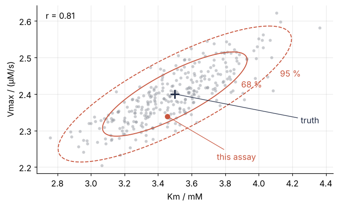
Fitted Vmax in µM/s against fitted Km in mM. Grey dots: 300 simulated assays, a cloud tilted upward with r = 0.81. Two outlines around the true constants: the 68 % and 95 % ellipses from this assay's covariance, which hold 72 % and 97 % of the dots. A red dot marks this assay's fit.

Of the 300 refits, 72 % fall inside the 68 % ellipse and 97 % inside the 95 % one. Report both errors and the correlation. The ratio \(V_\mathrm{max}/K_m\), or anything else computed from both, gets the wrong error without it.

Step 5: Recognize a failed fit

A fit that fails with an exception is the easy case. full_output=True makes curve_fit return three more things: infodict with diagnostics, mesg, a sentence on why the search stopped, and ier, a status code whose values 1 to 4 mean the search claims success. The helper prints one line per fit, and the cell fits the same assay four ways:

def report(label, popt, pcov, S, v, sigma):
    perr = np.sqrt(np.diag(pcov))
    chi2_dof = np.sum(((v - michaelis_menten(S, *popt)) / sigma) ** 2) / (S.size - popt.size)
    r = pcov[0, 1] / (perr[0] * perr[1])
    print(f"{label:4s} Vmax {popt[0]:6.3f} ± {perr[0]:.3f}  Km {popt[1]:6.3f} ± {perr[1]:.3f}"
          f"  chi2/dof {chi2_dof:6.2f}  r {r:.3f}")

report("(a)", popt, pcov, S, v, sigma)

# (b) a start with negative Km and no bounds
popt_b, pcov_b, infodict, mesg, ier = curve_fit(
    michaelis_menten, S, v, p0=[1, -1], sigma=sigma, absolute_sigma=True, full_output=True)
report("(b)", popt_b, pcov_b, S, v, sigma)
print("     ier =", ier, "  mesg:", " ".join(mesg.split()))

# (c) only the four concentrations below 2 mM
low = S < 2
popt_c, pcov_c = curve_fit(michaelis_menten, S[low], v[low], p0=p0, bounds=(0, np.inf),
                           sigma=sigma[low], absolute_sigma=True)
report("(c)", popt_c, pcov_c, S[low], v[low], sigma[low])

# (d) a budget of ten function calls
try:
    curve_fit(michaelis_menten, S, v, maxfev=10)
except RuntimeError as err:
    print("(d)  RuntimeError:", err)

(a)  Vmax  2.339 ± 0.076  Km  3.455 ± 0.284  chi2/dof   1.04  r 0.806
(b)  Vmax  0.100 ± 0.009  Km -1.017 ± 0.014  chi2/dof 240.49  r 0.786
     ier = 1   mesg: Both actual and predicted relative reductions in the sum of squares are at most 0.000000
(c)  Vmax  4.309 ± 3.802  Km  7.244 ± 7.485  chi2/dof   0.49  r 0.998
(d)  RuntimeError: Optimal parameters not found: Number of calls to function has reached maxfev = 10.

Line (b) is the dangerous one. ier is 1, the message says the sum of squares stopped shrinking, no warning appears, and the fit reports \(K_m = -1.017 \pm 0.014\) mM, a negative concentration with an error small enough to publish. Only chi-square per degree of freedom, 240 against 1.04 for the good fit, gives it away.

Line (c) passes that test, yet \(K_m = 7.2 \pm 7.5\) mM with a correlation of 0.998: far below \(K_m\) the law is a straight line of slope \(V_\mathrm{max}/K_m\), so four low points fix only the ratio. Line (d) is forced by a tiny budget, and it is the only failure that announces itself.

So check in this order: no exception, chi-square per degree of freedom near 1, parameters inside their bounds with finite, nonzero errors, and a correlation below about 0.95, above which the data barely tell the two parameters apart. Only then read the covariance. Without error bars the chi-square test is gone. Plot the residuals v - michaelis_menten(S, *popt) against S instead: they should fall above and below zero at random, and a long run of one sign means the model misses the shape of the data.

Step 6: Draw the fit over the data and check it against the truth

The figure from the beginning, from the weighted fit of Step 3, on a logarithmic concentration axis because the concentrations are spaced geometrically:

Vmax, Km = popt
S_fine = np.geomspace(0.3, 80, 300)
fig, ax = plt.subplots()
ax.axhline(Vmax, color=MUTED, lw=1, ls="--")
ax.plot([0.3, Km, Km], [Vmax / 2, Vmax / 2, 0], color=MUTED, lw=1, ls="--")
ax.plot(S_fine, michaelis_menten(S_fine, Vmax, Km), color=ACCENT)
ax.errorbar(S, v, yerr=sigma, fmt="o", color=INK, ms=4, capsize=2, lw=1)
ax.text(0.35, Vmax + 0.06, f"Vmax = {Vmax:.2f} ± {perr[0]:.2f} µM/s", color=INK)
ax.text(Km * 1.08, 0.12, f"Km = {Km:.2f} ± {perr[1]:.2f} mM", color=INK)
ax.text(12, 1.55, "curve_fit", color=ACCENT)
ax.set(xscale="log", xlim=(0.3, 80), ylim=(0, 2.75),
       xticks=[0.5, 1, 2, 5, 10, 20, 50], xticklabels=["0.5", "1", "2", "5", "10", "20", "50"],
       xlabel="S / mM", ylabel="v / (µM/s)")
plt.show()

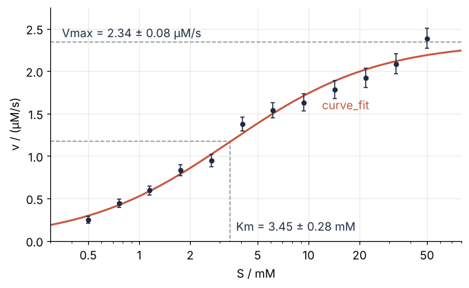
Initial rate in µM/s against substrate concentration in mM on a logarithmic axis. Dots with error bars: twelve measured rates. Line: the curve_fit result, rising to a dashed plateau at Vmax = 2.34 µM/s, with Km = 3.45 mM marked where the curve reaches half the plateau.

How far is the answer from the truth? The reciprocal plot of the motivation rests on

\[\frac{1}{v} = \frac{K_m}{V_\mathrm{max}}\,\frac{1}{S} + \frac{1}{V_\mathrm{max}} ,\]

so \(V_\mathrm{max}\) is one over the intercept and \(K_m\) is the slope times \(V_\mathrm{max}\). Both fits, measured in standard errors of the weighted fit:

slope, intercept = np.polyfit(1 / S, 1 / v, 1)
Vmax_lb, Km_lb = 1 / intercept, slope / intercept
for name, Vm, K in [("curve_fit", Vmax, Km), ("1/v against 1/S", Vmax_lb, Km_lb)]:
    print(f"{name:16s} Vmax = {Vm:.2f} µM/s ({(Vm - Vmax_true) / perr[0]:+.1f} SE)"
          f"   Km = {K:.2f} mM ({(K - Km_true) / perr[1]:+.1f} SE)")

curve_fit        Vmax = 2.34 µM/s (-0.8 SE)   Km = 3.45 mM (-0.2 SE)
1/v against 1/S  Vmax = 2.71 µM/s (+4.0 SE)   Km = 4.55 mM (+3.7 SE)

curve_fit is 0.8 standard errors below the true \(V_\mathrm{max}\) and 0.2 below the true \(K_m\), both inside one standard error, where about two assays in three land. The reciprocal line puts \(K_m\) at 4.55 mM and \(V_\mathrm{max}\) at 2.71 µM/s, 3.7 and 4.0 standard errors too high, from the same twelve rates. Fit the law as written.

Pitfalls

Starting values in the wrong units. Record the same assay in nM/s and the rates run up to 2,385, while the default start still puts \(V_\mathrm{max}\) at 1. The search has to cross three orders of magnitude and ends on negative constants without a warning, the quiet failure of line (b) in Step 5. The fix is the start of Step 2: v.max() and np.interp read the scale off whatever units the data are in, and bounds=(0, np.inf) forbids the negative answer.

absolute_sigma left at its default. With absolute_sigma=False, curve_fit multiplies pcov by chi-square per degree of freedom, so your sigmas set only the relative weights and their size drops out. Claim errors ten times larger than they are and compare:

for absolute in [False, True]:
    _, pcov_10 = curve_fit(michaelis_menten, S, v, p0=p0, bounds=(0, np.inf),
                           sigma=10 * sigma, absolute_sigma=absolute)
    print(f"absolute_sigma={absolute!s:5s}  error of Vmax = {np.sqrt(pcov_10[0, 0]):.3f} µM/s")

absolute_sigma=False  error of Vmax = 0.077 µM/s
absolute_sigma=True   error of Vmax = 0.760 µM/s

absolute_sigma=True reports ten times the honest 0.076 µM/s of Step 4, as it should. The default reports 0.077 µM/s: it dropped the factor of ten and scaled by the square root of chi-square per degree of freedom, 1.04 here. That it lands near the honest value is luck of this assay. On an assay whose error bars are too small, the default hides it. Set absolute_sigma=True whenever your sigmas are measured uncertainties.

A parameter the data cannot see. When changing a parameter does not change the curve over the range of your data, what you see depends on the method. Without bounds, where the method is "lm", curve_fit prints OptimizeWarning: Covariance of the parameters could not be estimated and fills all of pcov with inf. With bounds it says nothing: the idle parameter comes back exactly at its start with a standard error of 0, and the other errors look as healthy as before.

Give michaelis_menten an unused third argument, start it at 5, fit with the bounds and sigmas of Step 3, and you get 5.000 ± 0.000 next to the 0.076 µM/s and 0.284 mM of Step 4. A zero error does not mean a precise parameter; it means the fit never moved it.

So check that every entry of perr is finite and above zero and that popt differs from p0. In fits without bounds, make the warning stop the script: warnings.simplefilter("error", OptimizeWarning), with warnings from the standard library and OptimizeWarning from scipy.optimize, turns it into an exception. Then drop the parameter, or measure where it matters.

Variations

A confidence band around the curve. Propagate pcov through the model to shade where the true curve plausibly lies, as Fit a curve to data with error bars and draw a confidence band does with central differences.
Substrate inhibition. Some enzymes slow down again at high substrate: \(v = V_\mathrm{max} S/(K_m + S + S^2/K_i)\). Add Ki as a third argument, start it well above the largest \(S\), and bound it below by zero.
Cooperative binding. The Hill equation \(v = V_\mathrm{max} S^n/(K_{0.5}^n + S^n)\) adds the Hill coefficient \(n\). Start it at 1, where the law is Michaelis-Menten again.
Outliers. One bad well drags a least-squares fit. scipy.optimize.least_squares, the routine curve_fit calls when it has bounds, takes the residuals directly and with loss="soft_l1" gives large ones less pull.

Cheat sheet

def model(x, a, b): ...                       # x first, then one argument per parameter
popt, pcov, info, mesg, ier = curve_fit(
    model, x, y,
    p0=[a0, b0],                              # from the data, in its units; default is all ones
    bounds=([0, 0], [np.inf, np.inf]),        # switches the method from "lm" to "trf"
    sigma=s, absolute_sigma=True,             # no error bars: drop both; triplicates: s = SD / np.sqrt(3)
    full_output=True)                         # ier 1 to 4 claims success; mesg says why it stopped
chi2_dof = np.sum(((y - model(x, *popt)) / s) ** 2) / (len(x) - len(popt))   # near 1, or stop here
perr = np.sqrt(np.diag(pcov))                 # standard errors
corr = pcov / np.outer(perr, perr)            # above 0.95: the data cannot separate the parameters