Devito from the ground up: a seismic shot over a buried reflector

The problem: when does the echo from 500 m down arrive?

A seismic survey fires a source at the surface, a shot, and records the ground motion along a line of receivers. Say the top 500 m are water-saturated sediment, in which sound travels at 1,500 m/s, and below lies rock at 2,500 m/s. Straight below the source the echo from the interface comes back after 2 · 500 m / 1,500 m/s = 0.667 s. A receiver at horizontal distance \(x\) from the source, its offset, hears the echo after \(t(x) = \sqrt{x^2 + (2z)^2}\,/\,v\), with \(z\) = 500 m the depth and \(v\) = 1,500 m/s, a hyperbola.

Devito, a finite difference package from the seismic imaging community, checks this by simulation: you write the equation with SymPy, and Devito generates C, compiles it, and runs it. The equation is the acoustic wave equation with one extra term,

\[\frac{1}{v^2}\frac{\partial^2 u}{\partial t^2} - \nabla^2 u + \eta\,\frac{\partial u}{\partial t} = q ,\]

with \(u\) the pressure, \(v(x, z)\) the velocity, and \(q\) the source. The damping \(\eta\) is zero in the region we look at and nonzero only in a sponge around it, which Step 1 explains. For equal densities the interface reflects a fraction (2,500 − 1,500)/(2,500 + 1,500) = 0.25 of the incoming amplitude, with the same sign. Step 5 checks the time and the fraction.

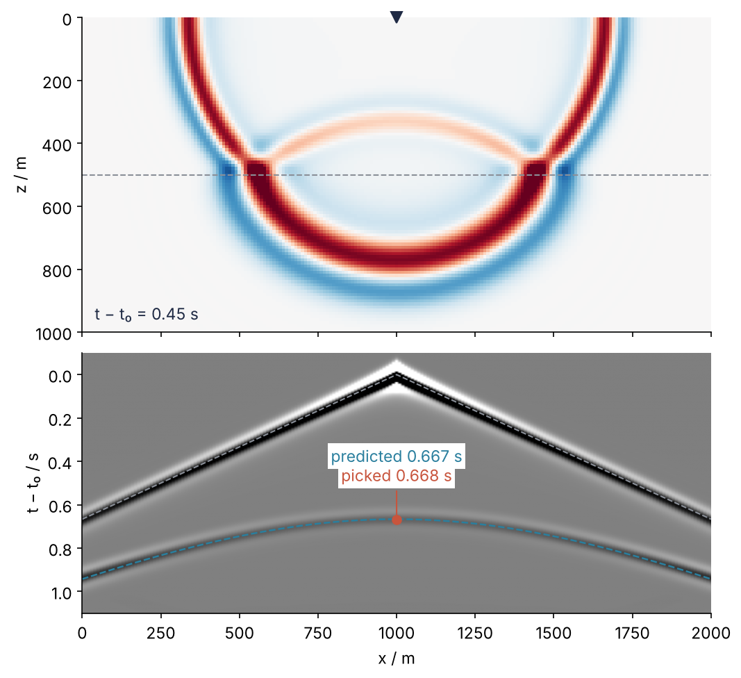
Top: pressure field 0.45 s after the source peak, depth 0 to 1,000 m against x 0 to 2,000 m, the echo on its way up from the interface at 500 m. Bottom: shot record, time against receiver position; the reflection hyperbola lies on the dashed prediction with its apex at 0.667 s.

The top panel is the pressure 0.45 s after the source peak, with the echo on its way up from the interface. The bottom panel is the shot record: every receiver's time series, its trace, side by side, with the predicted hyperbola drawn over it. Both come from one Operator run, and Step 6 draws them.

Setup

Devito installs with pip install devito and needs a C compiler, gcc or clang, because it compiles the code it writes. It knows no units. Everything below is in m, ms, and km/s, which is m/ms and the convention of Devito's own seismic examples, so that \(v\,\Delta t/\Delta x\) is a pure number as written.

import numpy as np
import matplotlib.pyplot as plt
from sympy import finite_diff_weights
# Devito's names one by one: "from devito import *" would replace Python's sum
from devito import (Grid, Function, TimeFunction, SparseTimeFunction, Eq, solve,
                    Operator, ConditionalDimension, configuration)

configuration["log-level"] = "WARNING"     # Devito otherwise logs run times, which change from run to run

v_sed, v_rock = 1.5, 2.5    # km/s, the same as m/ms
z_ref = 500.0               # depth of the interface, m
Lx, Lz = 2000.0, 1000.0     # the region we look at, m
dx = 10.0                   # grid spacing, m
nbl = 60                    # sponge width in grid points, on every side
f0 = 0.010                  # peak frequency of the source, kHz (10 Hz)

plt.rcParams.update({                      # the look of every figure below
    "figure.figsize": (7, 6), "figure.dpi": 110,
    "axes.spines.top": False, "axes.spines.right": False,
    "axes.grid": True, "grid.alpha": 0.25,
    "font.size": 11, "lines.linewidth": 1.8,
})
INK, ACCENT, SECOND, MUTED = "#1f2a44", "#c8553d", "#2a7f9e", "#8a8f98"

print(f"predicted zero-offset echo: {2 * z_ref / v_sed:.1f} ms")

predicted zero-offset echo: 666.7 ms

Step 1: Lay out the grid, the velocity model, and an absorbing sponge

Grid takes the number of points, the extent, and the origin. The 2,000 m × 1,000 m we care about get 60 extra points on every side, with the origin at (−600, −600) m so that the region of interest starts at (0, 0); z points down. The velocity is a Function: a SymPy symbol for the equations and a NumPy array, v.data, for the numbers (SymPy from the ground up covers the symbol side).

The padding exists because the grid ends. A wave reaching the last row bounces back as if from a wall the earth does not have, so a sponge damps it first. Two rules size it. Its width should exceed two dominant wavelengths at the fastest velocity, where they are longest: 2,500 m/s / 10 Hz = 250 m, so 600 m is 2.4 of them. Its strength rises as \(\eta_\text{max} d^2\), with \(d\) from 0 at the inner edge to 1 at the outer, because a sudden onset would itself reflect. The term \(\eta\,\partial u/\partial t\) makes the amplitude decay at the rate \(\eta v^2/2\), so a wave crossing a sponge of width \(W\) and coming back loses a factor \(e^{-\eta_\text{max} v W/3}\), with 1/3 the mean of \(d^2\) across the ramp. The slowest wave loses least, so \(\eta_\text{max} = 30/(v_\text{min} W)\) costs every wave at least a factor \(e^{-10}\).

shape = (int(Lx / dx) + 1 + 2 * nbl, int(Lz / dx) + 1 + 2 * nbl)
grid = Grid(shape=shape, extent=((shape[0] - 1) * dx, (shape[1] - 1) * dx),
            origin=(-nbl * dx, -nbl * dx))
x_ax = -nbl * dx + dx * np.arange(shape[0])     # x of every grid column, m
z_ax = -nbl * dx + dx * np.arange(shape[1])     # depth of every grid row, m
X, Z = np.meshgrid(x_ax, z_ax, indexing="ij")

v = Function(name="v", grid=grid)
v.data[:] = np.where(Z < z_ref, v_sed, v_rock)

W = nbl * dx
eta_max = 30 / (v_sed * W)                      # ms/m^2
d = np.maximum(np.maximum(-X, X - Lx), np.maximum(-Z, Z - Lz)) / W
damp = Function(name="damp", grid=grid)
damp.data[:] = eta_max * np.clip(d, 0, 1) ** 2

print(f"grid {grid.shape}, spacing {grid.spacing[0]:g} m")
print(f"v at z = 400 m: {v.data[160, 100]:.1f} km/s, at z = 600 m: {v.data[160, 120]:.1f} km/s")
print(f"damping at the center: {damp.data[160, 110]:.3f}, in a corner: {damp.data[0, 0]:.3f} ms/m^2")

grid (321, 221), spacing 10 m
v at z = 400 m: 1.5 km/s, at z = 600 m: 2.5 km/s
damping at the center: 0.000, in a corner: 0.033 ms/m^2

Of the 321 × 221 points, the 201 × 101 we record lie in the middle, where the sponge is exactly zero.

Step 2: Write the wave equation and let Devito solve it for the next step

The pressure changes in time, so it is a TimeFunction. A second time derivative by central differences needs \(u\) at \(t\) and at \(t - \Delta t\) to step to \(t + \Delta t\), the leapfrog scheme. The explicit Euler step of the heat equation tutorial needed only \(u\) at \(t\). time_order=2 asks for the extra level. space_order=8 asks for 9 points per direction in every spatial derivative: a wider stencil makes less error per cell, so fewer cells per wavelength suffice, and Pitfall 2 puts numbers on that.

u = TimeFunction(name="u", grid=grid, time_order=2, space_order=8)
print("u.data:", u.data.shape)

pde = u.dt2 / v**2 - u.laplace + damp * u.dt
stencil = Eq(u.forward, solve(pde, u.forward))
print(stencil)

u.data: (3, 321, 221)
Eq(u(t + dt, x, y), (-(-2.0*u(t, x, y)/dt**2 + u(t - dt, x, y)/dt**2)/v(x, y)**2 + Derivative(u(t, x, y), (x, 2)) + Derivative(u(t, x, y), (y, 2)) + damp(x, y)*u(t, x, y)/dt)/(damp(x, y)/dt + 1/(dt**2*v(x, y)**2)))

Three time levels, the oldest overwritten by the newest. solve replaced u.dt2 by a central difference, u.dt by a forward one, and rearranged the equation for \(u\) at \(t + \Delta t\), u.forward, the move the heat tutorial made by hand for one past level. The two space derivatives stay symbolic until the Operator writes them as 9-point stencils. Eq is an assignment, not an equation to solve: compute the right-hand side, store it in the left, at every grid point. Devito calls the second axis y; here it is the depth. The source \(q\) is missing, and Step 3 says why.

Step 3: Add a Ricker source and a line of receivers

The source is a Ricker wavelet, the standard pulse of seismic modeling: \((1 - 2a)\,e^{-a}\) with \(a = (\pi f_0 (t - t_0))^2\). It is delayed by \(t_0 = 1/f_0 = 100\) ms because a wavelet centered on \(t = 0\) would start already switched on. The time axis has 601 samples 2 ms apart, a step that Step 4 justifies.

Source and receivers may sit off the grid, each with its own time series: a SparseTimeFunction, one column per point. The source cannot go into pde: it is not a field on the grid. But in the solved equation \(u(t + \Delta t)\) carries the factor \(1/(v^2\Delta t^2)\), so a term \(q\) would add \(\Delta t^2 v^2 q\) to the new value (\(\eta\) is zero at the source). inject adds that to the grid points around the source after every update. interpolate is the reverse: it reads \(u\) at each receiver, one sample per receiver per step.

dt, nt = 2.0, 601                    # ms; 1,200 ms of record
t = np.arange(nt) * dt
t0 = 1 / f0                          # the wavelet's peak, ms
a = (np.pi * f0 * (t - t0)) ** 2
ricker = (1 - 2 * a) * np.exp(-a)

src = SparseTimeFunction(name="src", grid=grid, npoint=1, nt=nt)
src.coordinates.data[:] = [Lx / 2, 0.0]
src.data[:, 0] = ricker

rec = SparseTimeFunction(name="rec", grid=grid, npoint=201, nt=nt)
rec.coordinates.data[:, 0] = np.linspace(0, Lx, 201)     # one receiver every 10 m
rec.coordinates.data[:, 1] = 0.0

dt_sym = grid.time_dim.spacing       # the symbolic time step; the Operator fills it in at run time
src_term = src.inject(field=u.forward, expr=src * dt_sym**2 * v**2)
rec_term = rec.interpolate(expr=u)

print(f"src.data {src.data.shape}, rec.data {rec.data.shape}, wavelet peak at {t[np.argmax(ricker)]:.0f} ms")

src.data (601, 1), rec.data (601, 201), wavelet peak at 100 ms

Rows are time steps, columns points: rec.data[:, 100] is the trace at the source.

Step 4: Choose a stable time step and run the Operator

The limit on the time step comes from the fastest pattern a grid can hold, the sawtooth +1, −1, +1, … along an axis. The second-derivative stencil turns it into \(-S/\Delta x^2\) times itself, with \(S\) the sum of the absolute values of the stencil's weights. In two dimensions the two axes add, so the sawtooth obeys \(u'' = -\omega^2 u\) with \(\omega^2 = 2 S v^2/\Delta x^2\). Leapfrog on that oscillator stays bounded only for \(\omega\,\Delta t < 2\), a standard result I quote without proof, hence

\[\Delta t < \frac{2\,\Delta x}{v_\text{max}\sqrt{2S}} .\]

The heat tutorial's limit has the same origin, with a three-point stencil and \(S = 4\). SymPy's finite_diff_weights(2, range(-4, 5), 0) returns weights for derivatives up to order 2 on the points −4 … 4, evaluated at 0. Its last entry is the order-8 second derivative:

w = finite_diff_weights(2, range(-4, 5), 0)[-1][-1]
S = np.abs(np.array(w, dtype=float)).sum()
dt_max = 2 * dx / (v_rock * np.sqrt(2 * S))
print(f"S = {S:.4f}, dt_max = {dt_max:.4f} ms, dt = {dt:g} ms is {dt / dt_max:.2f} of it")

S = 6.5016, dt_max = 2.2185 ms, dt = 2 ms is 0.90 of it

The limit is set by the rock, not the sediment, and 2 ms uses 0.90 of it. An Operator takes the update, the injection, and the interpolation, and apply runs it. time_M=nt - 2 is the last step, the one that computes level nt − 1, and dt is a run-time argument:

op = Operator([stencil] + src_term + rec_term)
op.apply(time_M=nt - 2, dt=dt)

ccode = str(op.ccode).splitlines()
k = next(i for i, line in enumerate(ccode) if "u[t2][x + 8][y + 8] =" in line)
print(len(ccode), "lines of C; the innermost loop starts:")
for line in ccode[k - 4:k + 1]:
    print(line[:92])
print(f"largest |rec| = {np.abs(rec.data).max():.2f}, all finite: {np.isfinite(rec.data).all()}")

121 lines of C; the innermost loop starts:
      for (int y = y_m; y <= y_M; y += 1)
      {
        float r7 = 1.0F/(v[x + 1][y + 1]*v[x + 1][y + 1]);
        float r8 = -2.847222220F*u[t0][x + 8][y + 8];
        u[t2][x + 8][y + 8] = (-r7*(-2.0F*r1*u[t0][x + 8][y + 8] + r1*u[t1][x + 8][y + 8]) +
largest |rec| = 42.37, all finite: True

The first apply wrote those 121 lines of C and compiled them; later runs skip that. The line that assigns u[t2] is Step 2's solved stencil, with t0, t1, t2 the three time levels taking turns (no relation to the wavelet's \(t_0\)), and + 8 skips the 8-point halo of space_order=8. The record is finite, and its largest value, 42.37, is the direct wave next to the source.

Step 5: Read the reflection off the shot record

Near the source the direct wave dominates, so each pick searches within 60 ms of the prediction. The last pick is the direct wave at x = 0, which crosses the same 1,000 m of sediment as the zero-offset echo:

offset = rec.coordinates.data[:, 0] - Lx / 2
tau = t - t0                                          # time after the wavelet's peak, ms
print("offset   predicted   picked   amplitude")
for off in [0, 250, 500, 750]:
    t_pred = np.sqrt(off**2 + (2 * z_ref) ** 2) / v_sed
    trace = rec.data[:, np.argmin(np.abs(offset - off))]
    near = np.abs(tau - t_pred) < 60
    i = np.argmax(trace[near])
    print(f"{off:4.0f} m  {t_pred:7.1f} ms  {tau[near][i]:5.0f} ms  {trace[near][i]:9.2f}")
    if off == 0:
        t_pick0, a_pick0 = tau[near][i], trace[near][i]

near = np.abs(tau - 2 * z_ref / v_sed) < 60
i = np.argmax(rec.data[near, 0])
print(f"direct wave over 1,000 m: {tau[near][i]:.0f} ms, amplitude {rec.data[near, 0][i]:.2f}, "
      f"echo / direct = {a_pick0 / rec.data[near, 0][i]:.2f}")

offset   predicted   picked   amplitude
   0 m    666.7 ms    668 ms       0.76
 250 m    687.2 ms    690 ms       0.83
 500 m    745.4 ms    746 ms       1.06
 750 m    833.3 ms    834 ms       1.53
direct wave over 1,000 m: 674 ms, amplitude 2.93, echo / direct = 0.26

Every pick is within 3 ms of the hyperbola, but 668 against 666.7 ms is two errors that nearly cancel. The direct wave over the same 1,000 m peaks at 674 ms: a point source in two dimensions is a line source in three, and its pulse trails a tail that moves the peak late. The echo comes 6 ms earlier because on the grid the velocity jumps between the rows at 490 and 500 m, so the interface sits at 495 m and the round trip is 2 · 5 m / 1.5 km/s = 6.7 ms shorter. Like with like, the time agrees within a sample, and so does the amplitude, the spreading being equal: 0.26 against the predicted 0.25.

The table stops at the critical offset, 2 · 500 m · tan(asin(1.5/2.5)) = 750 m. Beyond it no wave enters the faster rock, the reflection is total and shifts its phase, and a head wave along the interface arrives first.

Step 6: Keep snapshots and draw the field with its shot record

A ConditionalDimension with factor=25 is a time index that advances once every 25 steps, 50 ms. A TimeFunction saved along it, filled by Eq(usave, u), keeps one field per 50 ms instead of all 601. Before the rerun u.data goes back to zero: its three time levels still hold the end of Step 4's run.

tsub = ConditionalDimension("tsub", parent=grid.time_dim, factor=25)
usave = TimeFunction(name="usave", grid=grid, time_order=0, save=nt // 25 + 1, time_dim=tsub)
op_snap = Operator([stencil] + src_term + rec_term + [Eq(usave, u)])

u.data[:] = 0
op_snap.apply(time_M=nt - 2, dt=dt)
record = np.array(rec.data)                           # a plain copy: the pitfalls below overwrite rec
k_snap = 11                                           # 11 * 50 ms = 550 ms, 450 ms after the peak
snap = np.array(usave.data[k_snap])
print(f"{usave.data.shape[0]} snapshots; snapshot {k_snap} is at t - t0 = {k_snap * 25 * dt - t0:.0f} ms")

25 snapshots; snapshot 11 is at t - t0 = 450 ms

inner = (slice(nbl, nbl + int(Lx / dx) + 1), slice(nbl, nbl + int(Lz / dx) + 1))
snap = snap[inner]
clip = np.percentile(np.abs(snap), 99.5)
clip_rec = np.percentile(np.abs(record), 98)
x_line = np.linspace(0, Lx, 401)

fig, (ax1, ax2) = plt.subplots(2, 1, sharex=True, figsize=(7, 6.4), height_ratios=[1, 0.8],
                               layout="constrained")
ax1.imshow(snap.T, extent=(-dx / 2, Lx + dx / 2, Lz + dx / 2, -dx / 2), cmap="RdBu_r",
           vmin=-clip, vmax=clip)                     # equal aspect: circles stay round
ax1.axhline(z_ref, color=MUTED, lw=1, ls="--")
ax1.plot(Lx / 2, 0, "v", color=INK, ms=8, clip_on=False)
ax1.text(40, 960, f"t − t₀ = {(k_snap * 25 * dt - t0) / 1000:.2f} s", color=INK)
ax1.set(ylabel="z / m", xlim=(0, Lx), ylim=(Lz, 0))
ax1.grid(False)

ax2.imshow(record, extent=(-dx / 2, Lx + dx / 2, (tau[-1] + dt / 2) / 1000, (tau[0] - dt / 2) / 1000),
           cmap="gray_r", vmin=-clip_rec, vmax=clip_rec, aspect="auto")
ax2.plot(x_line, np.abs(x_line - Lx / 2) / v_sed / 1000, color=MUTED, lw=1, ls="--")
ax2.plot(x_line, np.sqrt((x_line - Lx / 2) ** 2 + (2 * z_ref) ** 2) / v_sed / 1000,
         color=SECOND, lw=1.2, ls="--")
ax2.plot(Lx / 2, t_pick0 / 1000, "o", color=ACCENT, ms=6)
box = dict(boxstyle="square,pad=0.2", fc="white", ec="none")   # legible on the gray record
ax2.text(Lx / 2, 0.42, f"predicted {2 * z_ref / v_sed / 1000:.3f} s", ha="center", va="bottom",
         color=SECOND, bbox=box)
ax2.annotate(f"picked {t_pick0 / 1000:.3f} s", (Lx / 2, t_pick0 / 1000), xytext=(Lx / 2, 0.42),
             ha="center", va="top", color=ACCENT, bbox=box,
             arrowprops=dict(arrowstyle="-", color=ACCENT, lw=1))
ax2.set(xlabel="x / m", ylabel="t − t₀ / s", xlim=(0, Lx), ylim=(1.1, -0.1))
ax2.grid(False)
plt.show()

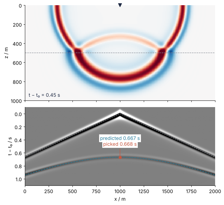
Top: pressure field 0.45 s after the source peak, depth 0 to 1,000 m against x 0 to 2,000 m, the echo on its way up from the interface at 500 m. Bottom: shot record, time against receiver position; the reflection hyperbola lies on the dashed prediction with its apex at 0.667 s.

RdBu_r shows positive pressure in red, negative in blue. The big ring is the direct wave, 675 m out. Below the dashed interface the transmitted front runs ahead in the faster rock, and the faint arc topping out near 325 m is the reflection on its way up. In the record the reflection lies on its dashed hyperbola, the direct wave on its dashed V.

Pitfalls

Echoes from the edges of the grid. The symptom is a strong event in the record that no layer explains. Rerun with no sponge, with Step 1's, and with one 7.5 times stronger, and look at the zero-offset trace after the echo has passed:

damp_good = damp.data.copy()
late = (tau > 750) & (tau < 1100)
for eta in [0.0, eta_max, 0.25]:
    damp.data[:] = damp_good * eta / eta_max
    u.data[:] = 0
    op.apply(time_M=nt - 2, dt=dt)
    late_amp = np.abs(rec.data[late, 100])            # receiver 100 sits at the source
    print(f"eta_max = {eta:.3f}: largest late amplitude {late_amp.max():.3f} at {tau[late][late_amp.argmax()]:.0f} ms")
damp.data[:] = damp_good

eta_max = 0.000: largest late amplitude 2.675 at 822 ms
eta_max = 0.033: largest late amplitude 0.045 at 752 ms
eta_max = 0.250: largest late amplitude 0.138 at 1090 ms

Without a sponge the top edge of the grid, 600 m above the source, sends back an echo due at 2 · 600 m / 1.5 km/s = 800 ms, its largest swing 3.5 times the reflection's 0.76. With Step 1's sponge, the 0.045 left at the very start of the window is the tail of the reflection itself. The sponge that is too strong reflects off its own steep rise: 0.138, three times as much, at the end of the window. Size it with Step 1's two rules, not by turning it up.

Too few grid points per wavelength. The symptom is a ringing tail behind each arrival, and arrivals slightly late. The Ricker spectrum falls to 3 % of its peak at 2.5 \(f_0\), so the shortest wavelength that matters is 1,500 m/s / 25 Hz = 60 m, 6 points at 10 m. Feed the stencil a wave \(\cos(kx)\) of wavenumber \(k\). The exact second derivative multiplies it by \(-k^2\), the stencil by \(\sum_j w_j \cos(jk\Delta x)/\Delta x^2\), a number closer to zero. Speed goes as the square root of that factor, so the square root of stencil factor over exact factor is the grid's speed as a fraction of the true speed, c in the code, with kh standing for \(k\Delta x\), \(2\pi\) over the points per wavelength:

for order in [2, 8]:
    j = list(range(-order // 2, order // 2 + 1))
    w_o = np.array(finite_diff_weights(2, j, 0)[-1][-1], dtype=float)
    kh = 2 * np.pi / np.array([6, 10, 18, 19])      # points per wavelength
    c = np.sqrt(-(w_o * np.cos(np.outer(kh, j))).sum(axis=1)) / kh
    print(f"order {order}: too slow by", "  ".join(f"{100 * (1 - ci):.3f} %" for ci in c))

order 2: too slow by 4.507 %  1.637 %  0.507 %  0.455 %
order 8: too slow by 0.018 %  0.000 %  0.000 %  0.000 %

At 6 points per wavelength order 2 carries the short waves 4.5 % too slowly, and they trail the pulse as that tail. Order 8 is off by 0.02 %. Order 2 is still 0.507 % slow at 18 points per wavelength and needs 19 to get under 0.5 %: 10 times as many grid points in two dimensions.

A time step over the limit. No error, just a record of NaN. Step 4's Operator takes dt at run time, so try both sides of the 2.2185 ms limit:

for dt_try in [2.2, 2.25]:
    u.data[:] = 0
    op.apply(time_M=nt - 2, dt=dt_try)
    print(f"dt = {dt_try} ms: NaN in the record: {np.isnan(rec.data).any()}")

dt = 2.2 ms: NaN in the record: False
dt = 2.25 ms: NaN in the record: True

A step 1.4 % over the limit loses the run without a word from Devito. Compute dt from the fastest velocity and the grid every time: a finer dx or a faster layer lowers it.

Variations

A dipping reflector. Fill v.data with np.where(Z < z_ref + np.tan(dip) * (X - Lx / 2), v_sed, v_rock). The apex of the hyperbola moves updip.
A lens or a salt body. Add a circle of 4.5 km/s with one more np.where, and recompute dt: v_max rises, so dt_max falls by 2.5/4.5, to 1.23 ms.
A free surface. Drop the top sponge, set u to zero on the row z = 0 with one more equation, and move source and receivers a few points down, where u is free to move. Ghosts appear, the source's upgoing wave sent back down, and multiples, waves bouncing between surface and interface.
A higher frequency. At \(f_0\) = 20 Hz the shortest wavelength halves, so dx must become 5 m, which halves dt_max. Four times the points for twice the steps: the run costs eight times as much.

Cheat sheet

grid = Grid(shape=(nx, nz), extent=(Lx_pad, Lz_pad), origin=(-W, -W))  # pad with a sponge, W > 2 wavelengths
v = Function(name="v", grid=grid); v.data[:] = ...                     # symbol and NumPy array at once
u = TimeFunction(name="u", grid=grid, time_order=2, space_order=8)     # leapfrog: three time levels
pde = u.dt2 / v**2 - u.laplace + damp * u.dt                           # damp = 30/(v_min W) * d**2 in the sponge
stencil = Eq(u.forward, solve(pde, u.forward))                         # solved for the next time level
src = SparseTimeFunction(name="src", grid=grid, npoint=1, nt=nt)       # off-grid points with time series
src_term = src.inject(field=u.forward, expr=src * grid.time_dim.spacing**2 * v**2)
rec_term = rec.interpolate(expr=u)                                     # rec.data[time, receiver]
dt = 0.9 * 2 * dx / (v_max * np.sqrt(2 * S))                           # S = sum |weights| of d2/dx2
Operator([stencil] + src_term + rec_term).apply(time_M=nt - 2, dt=dt)  # zero u.data before a rerun