PyVista for 3D fields: slices and isosurfaces through a block of rock

The problem: what shape is the dense body under the prospect?

A gravity survey over a prospect has been inverted into a 3D model of the ground below it. The model gives the density contrast, the density of the rock minus that of the host rock, in kg/m³, for every cell of a block 2,000 m by 2,000 m wide and 1,000 m deep. The block is cut into 100 × 100 × 50 cells of 20 m, half a million numbers. Somewhere in it sits rock 500 kg/m³ denser than its surroundings, and you want to know its shape.

The usual first look is a stack of 50 depth maps. On them a bright patch drifts sideways from map to map, and nobody can tell from the stack that it is one tilted lens. Matplotlib's 3D axes can stack the cells as cubes with voxels, but they cannot slice a volume or draw the surface on which the field takes one value, its isosurface, so they stop here too.

PyVista, a Python interface to VTK, the Visualization Toolkit, puts the array on a 3D grid and cuts it with filters: three orthogonal slices, a threshold that keeps the anomalous cells, and the isosurface at 250 kg/m³, half the contrast. The inversion smears the sharp edge of the body into a ramp from 0 to 500 kg/m³. Across a flat edge the ramp is symmetric, so its middle is where the edge was. Where the edge curves, the middle sits slightly inside, and Step 3 measures by how much.

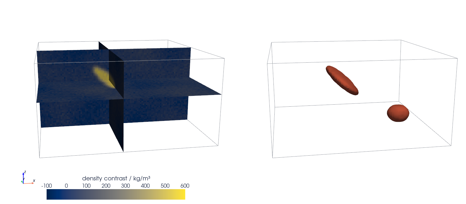
Two views of the same block of rock from the same camera. Left: three orthogonal slices colored by density contrast in cividis, dark blue host rock with a yellow streak where they cut the lens. Right: the 250 kg/m³ isosurface in red, a lens-shaped plate dipping about 40° to the right and a smaller round body deeper down, further right.

This is where we end up. The left half shows the slices, the right half the surface of the dense rock, both from one fixed camera, rendered off screen into a single PNG of 1600 × 700 px. The rest of this tutorial builds that figure.

Setup

Nothing here is drawn with Matplotlib, so there is no Matplotlib style block; PyVista takes the colormap by name and the palette as hex strings. The block below builds the model: a lens 1 km long and 140 m thick, tilted 40° down toward +x, and a smaller rounded body, both 500 kg/m³ denser than the host, softened at the edges and set on a smooth background with noise.

import numpy as np
import pyvista as pv
from scipy.ndimage import gaussian_filter

pv.OFF_SCREEN = True                 # render into memory, without a window;
pv.set_jupyter_backend("static")     # keep both in a notebook; in a desktop script, leave both out
                                     # and show() opens a window you can turn with the mouse

INK, ACCENT, SECOND, MUTED = "#1f2a44", "#c8553d", "#2a7f9e", "#8a8f98"
CMAP, CLIM = "cividis", (-100, 600)  # one color scale, in kg/m³, for every mesh
CAMERA = [(150, -3800, 600), (1000, 1000, -700), (0, 0, 1)]     # explained in Step 5
SBAR = dict(title="density contrast / kg/m³", fmt="%.0f", n_labels=8, color=INK, vertical=False,
            title_font_size=20, label_font_size=18, position_x=0.2, position_y=0.02, width=0.6, height=0.14)

NX, NY, NZ = 100, 100, 50            # cells
SPACING = 20.0                       # m
ORIGIN = (0.0, 0.0, -1000.0)         # m, the lower corner of the block; z up, 0 at the surface
x = ORIGIN[0] + SPACING * (np.arange(NX) + 0.5)    # cell centers
y = ORIGIN[1] + SPACING * (np.arange(NY) + 0.5)
z = ORIGIN[2] + SPACING * (np.arange(NZ) + 0.5)
X, Y, Z = np.meshgrid(x, y, z, indexing="ij")

def lens(center, a, b, c, dip):
    """Cells inside an ellipsoid with half-axes a along y, b down dip, c across, dipping toward +x."""
    d = np.radians(dip)
    u, v, w = X - center[0], Y - center[1], Z - center[2]
    s = u * np.cos(d) - w * np.sin(d)
    t = u * np.sin(d) + w * np.cos(d)
    return (v / a)**2 + (s / b)**2 + (t / c)**2 <= 1

ore = lens((900, 1000, -400), 500, 260, 70, 40) | lens((1500, 450, -720), 140, 140, 110, 0)
true_volume = 4 / 3 * np.pi * (500 * 260 * 70 + 140 * 140 * 110)    # m³

rng = np.random.default_rng(7)
rho = gaussian_filter(500.0 * ore, 1.0)              # an inversion smears the edges; sigma in cells
background = gaussian_filter(rng.standard_normal(ore.shape), 8)
rho += 30 * background / background.std() + 15 * rng.standard_normal(ore.shape)

print(f"rho: shape {rho.shape}, {rho.min():.0f} to {rho.max():.0f} kg/m³")
print(f"volume built into the model: {true_volume / 1e6:.1f} million m³")

rho: shape (100, 100, 50), -161 to 564 kg/m³
volume built into the model: 47.1 million m³

Step 1: Put the array on an ImageData grid

A field on a regular 3D lattice goes into pv.ImageData, a uniform grid described by three things: the position of its first point (origin), the distance between points (spacing), and the number of points along each axis (dimensions). Points are the corners of the cells, so 101 × 101 × 51 points bound 100 × 100 × 50 cells. The origin is the corner of the first cell, not its center: the density of the first cell belongs at x = 10 m, and the grid starts at 0.

grid = pv.ImageData(dimensions=(NX + 1, NY + 1, NZ + 1),
                    spacing=(SPACING, SPACING, SPACING), origin=ORIGIN)
grid.cell_data["drho"] = rho.ravel(order="F")
print(f"{type(grid).__name__}: {grid.n_cells} cells, {grid.n_points} points, dimensions {grid.dimensions}")
for axis, lo, hi in zip("xyz", grid.bounds[::2], grid.bounds[1::2]):
    print(f"  {axis} from {lo:6.0f} to {hi:5.0f} m")
print("first cell center / m:", grid.cell_centers().points[0])

ImageData: 500000 cells, 520251 points, dimensions (101, 101, 51)
  x from      0 to  2000 m
  y from      0 to  2000 m
  z from  -1000 to     0 m
first cell center / m: [  10.   10. -990.]

Half a million cells, 520,251 points, and the block where it should be: z from -1,000 m to the surface, the first cell's center at (10, 10, -990) m.

The order="F" in that cell is the line that matters. A grid stores its values as one long list, and ravel writes the 3D array into such a list. The order says which index changes from one entry to the next, the way the last digit of an odometer turns fastest. NumPy's default, C order, steps the last index first, here z. VTK expects x, the first index, to step first, which is how Fortran stores arrays, hence "F". On a small array:

a = np.arange(8).reshape(2, 2, 2)
print("C order:", a.ravel())
print("F order:", a.ravel(order="F"))

C order: [0 1 2 3 4 5 6 7]
F order: [0 4 2 6 1 5 3 7]

Get it wrong and nothing complains, because the length is the same. Ask both grids for the cell at the center of the lens:

wrong = grid.copy()
wrong.cell_data["drho"] = rho.ravel()               # NumPy's default, C order
i = grid.find_closest_cell((900, 1000, -400))
print(f"at the lens center: order='F' {grid['drho'][i]:5.0f} kg/m³,  C order {wrong['drho'][i]:5.0f} kg/m³")

at the lens center: order='F'   515 kg/m³,  C order    -5 kg/m³

The right grid finds 515 kg/m³, the dense rock; the wrong one finds -5 kg/m³, background, because it has scattered the lens across the block. For an array indexed [ix, iy, iz], the rule is ravel(order="F"), every time.

Step 2: Cut three orthogonal slices

slice_orthogonal cuts the grid with three planes, one perpendicular to each axis, through a point you choose. Through the lens center:

slices = grid.slice_orthogonal(x=900, y=1000, z=-400)
print(f"{type(slices).__name__} of {slices.n_blocks} meshes:",
      ", ".join(f"{name} plane {block.n_cells} cells" for name, block in zip(slices.keys(), slices)))

MultiBlock of 3 meshes: YZ plane 5000 cells, XZ plane 5000 cells, XY plane 10000 cells

The result is a MultiBlock, a container that holds several meshes, here one per plane. Every picture in PyVista is made the same way: create a Plotter, add meshes to it with add_mesh, then call show() or screenshot(). Since three steps draw one mesh each from the same camera, a small function does it, with the edges of the block in MUTED for orientation. The colormap is cividis, for the reasons given in Colormaps: why a rainbow scale draws features that are not in the data.

def show(mesh, **style):
    pl = pv.Plotter(window_size=(900, 700))
    pl.set_background("white")
    pl.add_mesh(mesh, **style)
    for bar in pl.scalar_bars.values():          # none for a single-color mesh; see Step 5
        bar.GetTitleTextProperty().SetLineOffset(-10)
    pl.add_mesh(grid.outline(), color=MUTED)
    pl.camera_position = CAMERA
    pl.show()

show(slices, scalars="drho", cmap=CMAP, clim=CLIM, scalar_bar_args=SBAR)

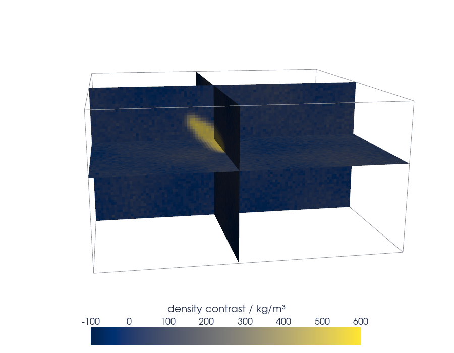
Three orthogonal slices through a block of rock, colored by density contrast from -100 to 600 kg/m³ in cividis. The host rock is dark blue; the lens shows only as a yellow streak, dipping to the right, near the point where the three planes meet.

The lens is the yellow streak, at its brightest about 500 kg/m³ above the dark blue host rock, and it shows only where a plane happens to cut it. That is all three planes can say. No plane passes through the second body, so the picture has no trace of it.

Step 3: Keep the anomalous cells with threshold

threshold(250, scalars="drho") keeps every cell whose value is 250 or more and drops the rest. The result is an UnstructuredGrid, a mesh of whole cells in no particular arrangement, and it knows its own volume. connectivity() labels each group of touching cells with a number, its RegionId, so counting the labels counts the bodies:

ore_cells = grid.threshold(250, scalars="drho")
bodies = ore_cells.connectivity()
print(f"{type(ore_cells).__name__} with {ore_cells.n_cells} cells")
print(f"volume above 250 kg/m³: {ore_cells.volume / 1e6:.1f} million m³, built: {true_volume / 1e6:.1f} million m³, "
      f"difference {ore_cells.volume / true_volume - 1:+.1%}")
print(f"separate bodies: {len(np.unique(bodies['RegionId']))}, cells in each: {np.bincount(bodies.cell_data['RegionId'])}")

UnstructuredGrid with 5744 cells
volume above 250 kg/m³: 46.0 million m³, built: 47.1 million m³, difference -2.5%
separate bodies: 2, cells in each: [4710 1034]

Two bodies, and a volume that agrees with the one built into the model to 2.5 %. That is the check on the half-contrast level. The shortfall is the curvature. Smearing averages each cell with its neighbors, and at the edge of a convex body fewer than half of them lie inside, so the edge ends up below 250 kg/m³ and the half level moves inward. The thinner the body compared with the smearing, the more it shrinks. The kept cells, colored by their value:

show(ore_cells, scalars="drho", cmap=CMAP, clim=CLIM, scalar_bar_args=SBAR)

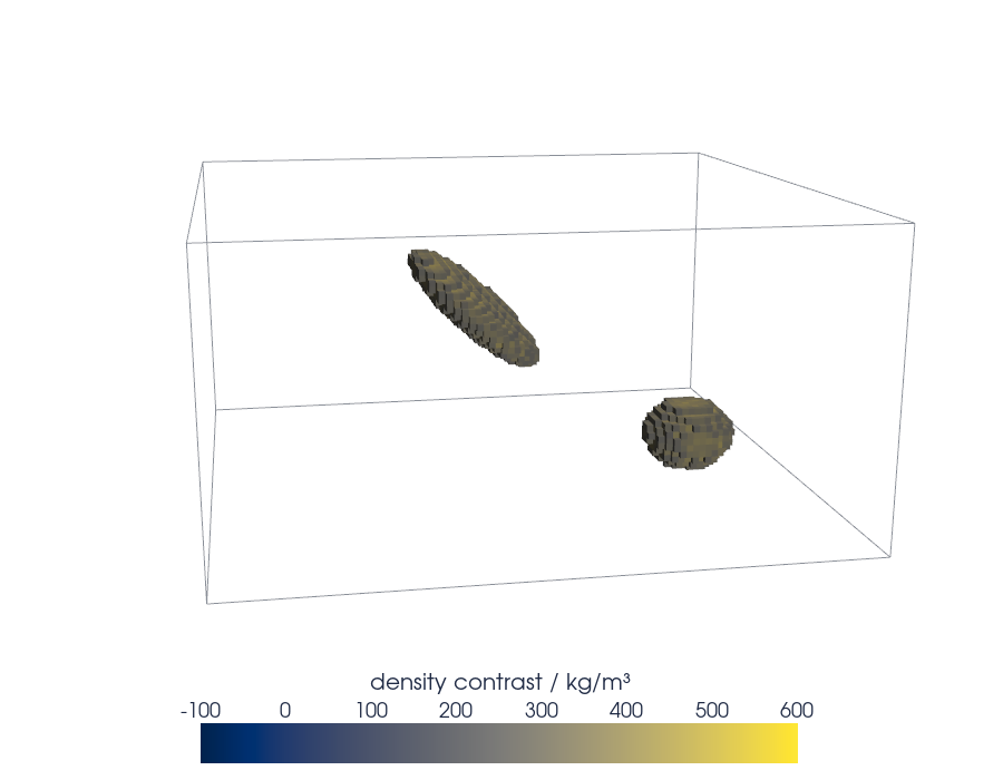
The cells of the block with a density contrast of 250 kg/m³ or more, drawn as blocks of 20 m in cividis: a lens-shaped plate dipping about 40° to the right and a smaller rounded body deeper down, further right, inside the outline of the block.

The second body, which the slices in Step 2 missed, is there, and the lens is a staircase of 20 m blocks. The volume is honest; the surface is not something you would put in a paper.

Step 4: Draw the isosurface with contour

The isosurface is built from triangles; in two dimensions it would be a contour line, which is why PyVista calls the filter contour. On the grid as it is, it refuses:

try:
    grid.contour([250], scalars="drho")
except TypeError as err:
    print("TypeError:", err)

TypeError: Contour filter only works on point data.

Contouring interpolates between the corners of cells, so it needs values on the points. cell_data_to_point_data() gives each point the average of the cells that share it, eight inside the block and fewer on its faces. The field is the same data smoothed over one cell, so the peak drops a little.

pt = grid.cell_data_to_point_data()
print(f"maximum: cells {rho.max():.0f} kg/m³, points {pt['drho'].max():.0f} kg/m³")

iso = pt.contour([250], scalars="drho")
print(f"{iso.n_cells} triangles, area {iso.area / 1e6:.2f} km², enclosing {iso.volume / 1e6:.1f} million m³")

maximum: cells 564 kg/m³, points 534 kg/m³
7596 triangles, area 1.05 km², enclosing 45.0 million m³

The peak lost 30 kg/m³ of 564. The surface encloses 45.0 million m³ against the 46.0 the threshold kept. Part of that is the averaging, a second smearing that moves the half level inward as in Step 3; the rest is the triangles, which cut corners that the threshold keeps whole. Spread over 1.05 km² of surface, the 1.0 million m³ is a layer under 1 m thick, a twentieth of a cell. Threshold and isosurface describe the same body.

show(iso, color=ACCENT, smooth_shading=True)

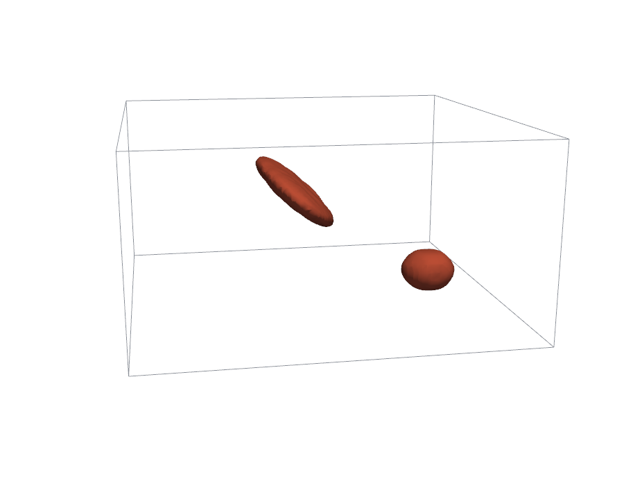
The 250 kg/m³ isosurface in red with smooth shading, inside the outline of the block: a lens-shaped plate dipping about 40° to the right and a smaller rounded body deeper down, further right.

The lens is one smooth plate dipping about 40° toward +x, and the second body is a separate lump deeper down and off to the side. This is the picture the stack of depth maps could not give: one object where the maps showed a patch drifting from map to map.

Step 5: Fix the camera and the colorbar

The final figure puts the slices and the isosurface side by side in one window. Plotter(shape=(1, 2)) makes two viewports, subplot picks the one that the next meshes go into, and link_views() makes both share one camera, so turning one turns the other.

pl = pv.Plotter(shape=(1, 2), window_size=(1600, 700), border=False)
pl.set_background("white")
pl.subplot(0, 0)
pl.add_mesh(slices, scalars="drho", cmap=CMAP, clim=CLIM, scalar_bar_args=SBAR)
pl.scalar_bar.GetTitleTextProperty().SetLineOffset(-10)
pl.add_mesh(grid.outline(), color=MUTED)
pl.add_axes(color=INK)
pl.subplot(0, 1)
pl.add_mesh(iso, color=ACCENT, smooth_shading=True)
pl.add_mesh(grid.outline(), color=MUTED)
pl.link_views()
pl.camera_position = CAMERA
print(pl.camera_position)

[(150.0, -3800.0, 600.0),
 (1000.0, 1000.0, -700.0),
 (0.0, 0.0, 1.0)]

A camera position is three tuples: the point it stands at, the point it looks at, and the direction that is up on the screen, all in the units of the grid. CAMERA stands 600 m above the surface and 3.8 km in front of the y = 0 face, near x = 150 m, and looks at (1000, 1000, -700) m along the strike of the lens, the +y direction. Along strike you lose the 1 km length of the lens and see its dip.

Aiming below the lens lifts the block clear of the colorbar. Every figure here used this camera, which is why they line up. To find your own, run the plot as a script on a desktop without the two rendering lines of Setup, turn the view with the mouse, and keep what pl.show(return_cpos=True) returns.

The colorbar takes its look from scalar_bar_args: the title with its unit, horizontal, labels formatted as whole numbers, eight of them so they fall every 100 kg/m³, font sizes in pixels, and text in INK. VTK sets the title flush on the labels, and PyVista has no option for the gap, so the code calls the VTK object underneath, hence the CamelCase: SetLineOffset(-10) lifts the title by 10 px. The colors mean the same in every panel only because every mesh got the same clim.

Step 6: Render off screen to a PNG at a set size

screenshot renders the window and returns the pixels as an array; give it a file name and it writes a PNG as well.

img = pl.screenshot()
print("image array:", img.shape)
pl.show()

image array: (700, 1600, 3)

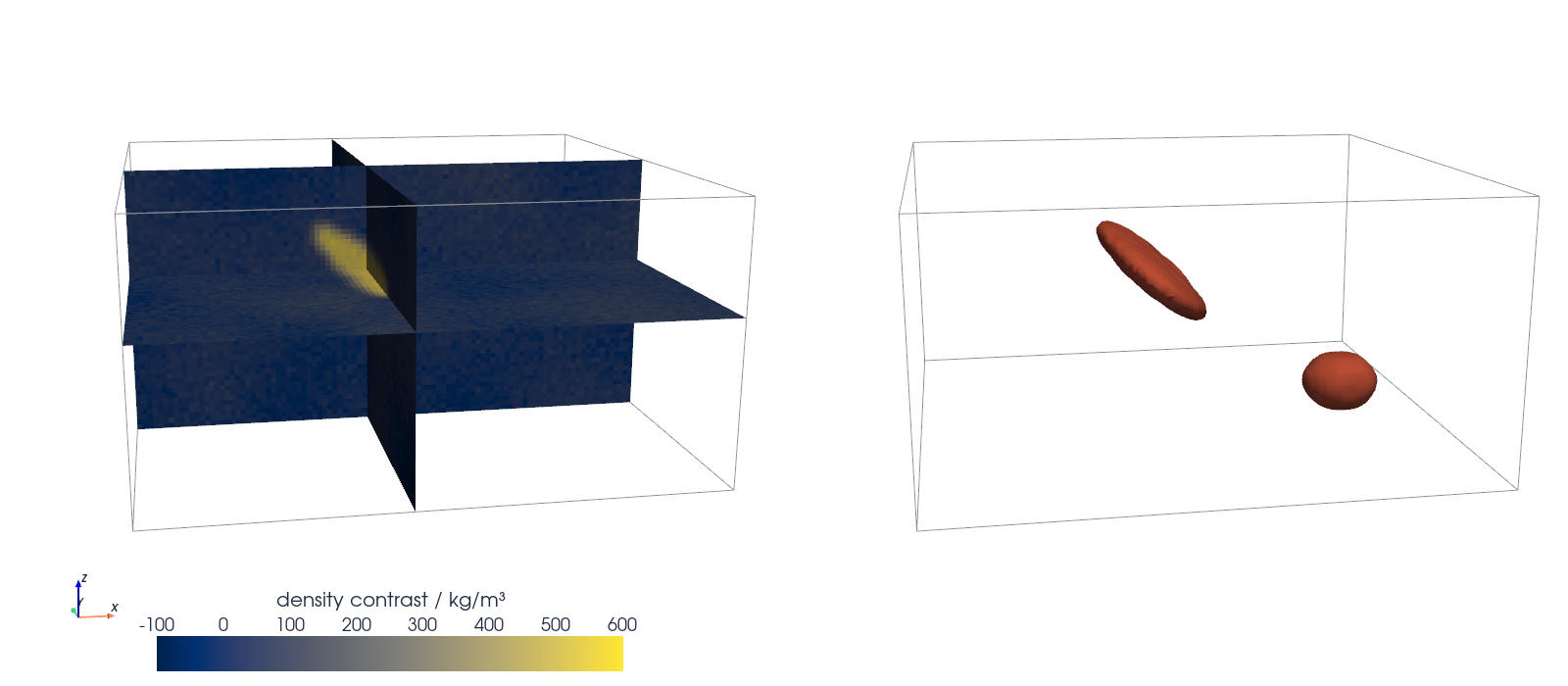
Two views of the same block from the same camera. Left: three slices in cividis with a horizontal colorbar from -100 to 600 kg/m³ and a yellow streak at the lens. Right: the 250 kg/m³ isosurface in red, the lens as a plate dipping about 40° to the right and a smaller round body deeper down.

The array is 700 rows by 1600 columns by three colors, exactly the window_size. For a print version, pl.screenshot(path, scale=2) renders at 3200 × 1400 px with fonts and lines scaled alike, enough for a figure 8 inches wide at 400 dpi. The figure at the top of this page is the same call with a file name, and two executions of this notebook write byte-identical PNGs, so the figure is as reproducible as the numbers.

Pitfalls

Points or cells, off by one. It is natural to pass the array's shape as dimensions, but that makes 100 × 100 × 50 points, which bound only 99 × 99 × 49 cells:

short = pv.ImageData(dimensions=rho.shape, spacing=(SPACING, SPACING, SPACING), origin=ORIGIN)
try:
    short.cell_data["drho"] = rho.ravel(order="F")
except ValueError as err:
    print("ValueError:", str(err).splitlines()[0])

ValueError: Invalid array shape. Array 'drho' has length (500000) but a length of (480249) was expected.

The same values assigned to point_data fit without complaint and sit every value half a cell away from where it belongs. For one value per cell, the dimensions are the shape plus one. Point data is right when the values were sampled at nodes, as in a finite-difference solution or a temperature grid from a model: then dimensions=rho.shape, origin at the first sample, and point_data, and contour works without the conversion of Step 4. The mistake is putting cell values on points, not using points.

Each mesh gets its own color range. Leave out clim, and add_mesh stretches the colormap over the values of that mesh alone:

for name, mesh in [("slices", slices), ("threshold", ore_cells)]:
    lo, hi = mesh.get_data_range("drho")
    print(f"{name:9s} {lo:5.0f} to {hi:4.0f} kg/m³")

slices     -115 to  564 kg/m³
threshold   250 to  564 kg/m³

The darkest blue would mean -115 kg/m³ on the slices and 250 kg/m³ on the kept cells, and a single colorbar would lie about one of them. One clim for every mesh that shares a colorbar.

A blank window or a crash on a server. On a cluster node or in a CI job there is no display, VTK cannot open a window, and the notebook hangs or dies. pv.OFF_SCREEN = True is half the fix. The other half is an OpenGL library that renders without a display, OSMesa or EGL, which on Debian and Ubuntu come as the system packages libosmesa6 and libegl1. This notebook was executed on such a machine.

Variations

Volume rendering. pl.add_volume(grid, cmap=CMAP, opacity="sigmoid") instead of a surface, for a field without a sharp edge, such as a plume or a temperature field.
Nested shells. pt.contour([150, 250, 400]) with opacity=0.3 on the outer ones shows how sharp the edge of the body is.
A cut-away block. grid.clip(normal="y", origin=(900, 1000, -400), invert=False) removes the half of the block nearest the camera and leaves the block diagram geologists draw by hand; clip_box cuts out a corner.
Cells that grow with depth, or a finite-element mesh. pv.RectilinearGrid(x, y, z) takes an inversion mesh with padding cells, pv.read("part.vtu") the stress in a machined part. The filters are the same.

Cheat sheet

grid = pv.ImageData(dimensions=np.array(a.shape) + 1,  # points = cells + 1
                    spacing=(dx, dy, dz), origin=corner)
grid.cell_data["f"] = a.ravel(order="F")               # x runs fastest
slices = grid.slice_orthogonal(x=x0, y=y0, z=z0)       # MultiBlock of three planes
kept = grid.threshold(level, scalars="f")              # whole cells, f >= level
iso = grid.cell_data_to_point_data().contour([level], scalars="f")
pl = pv.Plotter(off_screen=True, window_size=(1600, 700))
pl.add_mesh(slices, scalars="f", cmap="cividis", clim=(lo, hi))   # same clim everywhere
pl.camera_position = [position, focal_point, view_up]
pl.screenshot("figure.png", scale=2)                   # pixels times two, fonts too