Dynamic light scattering: nanoparticle size from the flicker of laser light (Python)

The problem: particle size from the flicker of a laser speckle

Shine a 633 nm laser through a drop of water with 100 nm plastic spheres in it and put a photon counter at 90°. The scattered light interferes into speckle, a grainy pattern of bright and dark spots, and the counter sits in one spot, one coherence area. The spheres diffuse, the speckle rearranges, and the count rate flickers within half a millisecond. Dynamic light scattering (DLS) turns that flicker into a size. It is behind most nanoparticle, protein, and micelle sizes in chemistry and biochemistry, and the one number the instrument prints is only as good as the fit to the curve behind it.

A sphere of diameter \(d\) in a liquid of viscosity \(\eta\) diffuses with the Stokes-Einstein coefficient \(D = k_B T/(3\pi\eta d)\), which for 100 nm in water at 25 °C is 4.91 × 10⁻¹² m²/s. The detector at the angle \(\theta\) watches one length scale, set by the scattering vector \(q = (4\pi n/\lambda)\sin(\theta/2)\) with \(n = 1.33\) the refractive index of water. At 90° that is \(q = 1.867 \times 10^{7}\) m⁻¹: the pattern repeats every \(2\pi/q \approx 340\) nm and has changed once a particle has moved about \(1/q \approx 54\) nm. Diffusing a distance \(x\) takes a time \(x^2/D\), so the speckle forgets itself at the rate

\[\Gamma = Dq^2 ,\]

which is 1,711 s⁻¹, once every 0.585 ms. Another angle watches another length, which one of the variations uses.

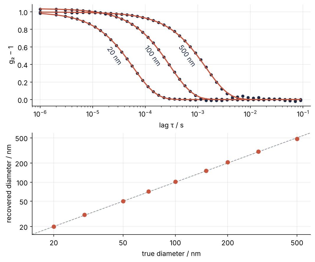
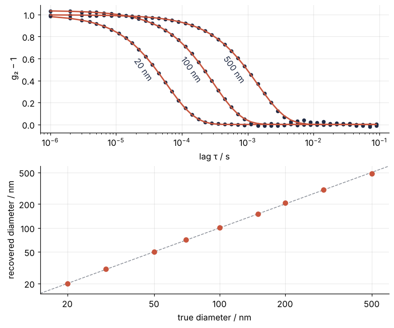
Top: intensity correlation g2 − 1 against lag in s, log axis, for 20, 100, and 500 nm spheres; the smaller the particle, the earlier the decay. Bottom: recovered diameter against true diameter for nine samples from 20 to 500 nm, all on the diagonal.

Smaller particles decay sooner, and the sizes read back land on the diagonal. Each point is one simulated trace of photon counts, turned into its autocorrelation with the FFT and fitted with curve_fit.

Setup

The constants describe the sample of the problem; diffusion and diameter are Stokes-Einstein in both directions.

import numpy as np
import matplotlib.pyplot as plt
from scipy.signal import lfilter
from scipy.optimize import curve_fit

kB = 1.380649e-23          # J/K
T = 298.15                 # K
eta = 0.89e-3              # Pa s, water at 25 °C
n_medium = 1.33            # refractive index of water
wavelength = 633e-9        # m
theta = np.radians(90)     # detector angle
q = 4 * np.pi * n_medium * np.sin(theta / 2) / wavelength

def diffusion(d):
    return kB * T / (3 * np.pi * eta * d)

def diameter(gamma):
    return kB * T * q**2 / (3 * np.pi * eta * gamma)

dt = 1e-6                  # s, sample time of the counter
N = 2**22                  # samples per measurement, 4.19 s
rate = 5e5                 # mean count rate, photons/s
rng = np.random.default_rng(276)

plt.rcParams.update({
    "figure.figsize": (7, 3.6), "figure.dpi": 110,
    "axes.spines.top": False, "axes.spines.right": False,
    "axes.grid": True, "grid.alpha": 0.25,
    "font.size": 11, "lines.linewidth": 1.8,
})
INK, ACCENT, SECOND, MUTED = "#1f2a44", "#c8553d", "#2a7f9e", "#8a8f98"

gamma_100 = diffusion(100e-9) * q**2
print(f"q = {q:.4g} 1/m   D(100 nm) = {diffusion(100e-9):.3g} m²/s   "
      f"Γ = {gamma_100:,.0f} 1/s   1/Γ = {1e3 / gamma_100:.3f} ms")

q = 1.867e+07 1/m   D(100 nm) = 4.91e-12 m²/s   Γ = 1,711 1/s   1/Γ = 0.585 ms

Step 1: Simulate the scattered light as a Gaussian field

The field at the detector is the sum of the waves from many particles, each with a random phase. A sum of many independent contributions is Gaussian, so the field \(E\) is a complex Gaussian number, and the counter sees its intensity \(|E|^2\). Each particle's phase random-walks as it diffuses, and the field forgets its past exponentially: a lag \(\tau\) later it keeps on average a fraction \(g_1(\tau) = e^{-\Gamma\tau}\) of its present value.

Sampled every \(\Delta t\), such a field obeys a one-line recursion,

\[E_{k+1} = \rho\,E_k + \sqrt{1-\rho^2}\,\xi_k , \qquad \rho = e^{-\Gamma\Delta t},\]

with \(\xi_k\) complex standard normal noise. Each sample keeps a fraction \(\rho\) of the last one and adds fresh noise, sized so that the mean intensity stays 1. (This is an AR(1), or sampled Ornstein-Uhlenbeck, process.) scipy.signal.lfilter(b, a, x) runs exactly such a recursion over a whole array, so there is no Python loop over 4 million samples. It keeps the output terms on the left, \(a_0 E_{k+1} + a_1 E_k = b_0 \xi_k\), so the recursion above is a = [1, -rho] and b = [sqrt(1 - rho**2)]. The counter then records a Poisson number of photons per sample, with mean rate × \(|E|^2\) × \(\Delta t\), about 0.5.

def scattered_field(gamma):
    rho = np.exp(-gamma * dt)
    xi = (rng.standard_normal(N) + 1j * rng.standard_normal(N)) / np.sqrt(2)
    return lfilter([np.sqrt(1 - rho**2)], [1, -rho], xi)

def photon_counts(field):
    return rng.poisson(rate * dt * np.abs(field)**2)

# full-length traces, as a measurement would make them; only 10 ms are plotted
fields = {d: scattered_field(diffusion(d * 1e-9) * q**2) for d in (20, 500)}
t_ms = np.arange(10_000) * dt * 1e3

fig, axes = plt.subplots(2, 1, figsize=(7, 4.2), sharex=True, sharey=True)
for ax, (d, E) in zip(axes, fields.items()):
    ax.plot(t_ms, np.abs(E[:10_000])**2, color=INK, lw=1.2)
    ax.text(0.99, 0.92, f"{d} nm", transform=ax.transAxes, ha="right", va="top")
    ax.set(ylabel="|E|²")
axes[1].set(xlabel="t / ms", xlim=(0, 10))
plt.show()

for d, E in fields.items():
    print(f"{d:3d} nm: Γ = {diffusion(d * 1e-9) * q**2:7,.0f} 1/s   mean |E|² = {np.mean(np.abs(E)**2):.3f}")

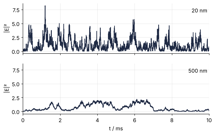
Scattered intensity |E|² against time in ms over the first 10 ms. Top: 20 nm spheres, a dense flicker of narrow spikes. Bottom: 500 nm spheres, a few slow swells. Both fluctuate around a mean of 1.

 20 nm: Γ =   8,553 1/s   mean |E|² = 0.996
500 nm: Γ =     342 1/s   mean |E|² = 0.993

The 20 nm field flickers 25 times faster than the 500 nm field, the ratio of their decay rates, and both fluctuate around the mean intensity of 1.

Step 2: Autocorrelate the photon counts with the FFT

What an instrument computes from the counts \(n\) is the intensity autocorrelation,

\[g_2(\tau) = \frac{\langle n(t)\,n(t+\tau)\rangle}{\langle n\rangle^2},\]

the average product of the count now and the count a lag \(\tau\) later, normalized so that it is 1 when the two are unrelated. Done directly at every lag, that is \(N^2 \approx 1.8 \times 10^{13}\) multiplications. The FFT does it in \(N \log N\) through the Wiener-Khinchin theorem: the squared magnitude \(|F|^2\) of the Fourier transform of the counts, transformed back, is their correlation at every lag at once. One catch: the FFT treats the trace as periodic, so its end wraps onto its start and the long lags mix with the short ones. Padding with \(N\) zeros, a transform of length \(2N\), makes the correlation linear instead of circular. At lag \(k\) only \(N - k\) pairs overlap, so the sum is divided by \(N - k\).

def autocorrelate(counts):
    x = counts.astype(float)
    F = np.fft.rfft(x, 2 * len(x))                  # zero-padded to 2N
    acf = np.fft.irfft(np.abs(F)**2)[:len(x)] / (len(x) - np.arange(len(x)))
    return acf / x.mean()**2

counts = photon_counts(scattered_field(gamma_100))
g2 = autocorrelate(counts)
print(f"mean counts per sample {counts.mean():.3f}")
for k in range(4):
    print(f"g2({k} µs) = {g2[k]:.3f}")
print(f"g2 averaged over 50 to 100 ms = {g2[50_000:100_001].mean():.4f}")

mean counts per sample 0.501
g2(0 µs) = 4.001
g2(1 µs) = 2.009
g2(2 µs) = 2.004
g2(3 µs) = 2.003
g2 averaged over 50 to 100 ms = 1.0002

At lag 0 the correlation is 4.00, not 2. Every photon is correlated with itself: a Poisson count has a variance equal to its mean, and that shot noise adds \(1/(\text{rate}\,\Delta t) = 2\) at lag 0 and nowhere else. One microsecond later \(g_2\) is 2.01, the value of Gaussian light, whose \(\langle I^2\rangle = 2\langle I\rangle^2\), and at long lags it is 1.000. Lag 0 is dropped from here on.

Step 3: Average onto a logarithmic lag grid

The decay is over by 1 ms, yet 99 % of the 100,000 lags up to 0.1 s lie beyond it, and a fit on that grid would fit the baseline. Instruments report logarithmically spaced lags instead, straight from their multi-tau hardware correlators. Averaging the linear-lag result over bins, ten per decade, gives the same grid. The sum of \(g_2\) over a bin is the difference of the running sum at its two edges, so every bin mean costs two lookups, and the lag of a bin is the mean of its lags.

edges = np.unique(np.round(np.logspace(0, 5, 51)).astype(int))   # lags in samples

def log_bin(g2):
    running = np.concatenate([[0], np.cumsum(g2)])
    running_lag = np.concatenate([[0], np.cumsum(np.arange(len(g2)))])
    width = np.diff(edges)
    tau = (running_lag[edges[1:]] - running_lag[edges[:-1]]) / width * dt
    return tau, (running[edges[1:]] - running[edges[:-1]]) / width

tau, g2_binned = log_bin(g2)
lag = np.arange(1, edges[-1]) * dt
g2_lag = g2[1:edges[-1]]

fig, ax = plt.subplots()
ax.plot(lag, g2_lag - 1, color=INK, lw=0.8, alpha=0.3)
ax.plot(tau, g2_binned - 1, "o", color=INK, ms=4)
ax.set(xscale="log", xlabel="lag τ / s", ylabel="g₂ − 1", xlim=(7e-7, 0.14))
plt.show()

late, late_bins = lag > 0.01, tau > 0.01
spread = np.std(g2_lag[late])
print(f"{len(tau)} bins from {tau[0] * 1e6:.0f} µs to {tau[-1] * 1e3:.0f} ms")
print(f"spread past 10 ms   single lags ±{spread:.4f}")
# a difference of two independent errors is √2 times one of them
print(f"                    new at each lag ±{np.std(np.diff(g2_lag[late])) / np.sqrt(2):.4f}")
print(f"                    bins ±{np.std(g2_binned[late_bins]):.4f}, "
      f"if the lags were independent ±{spread / np.sqrt(np.diff(edges)[late_bins].mean()):.4f}")

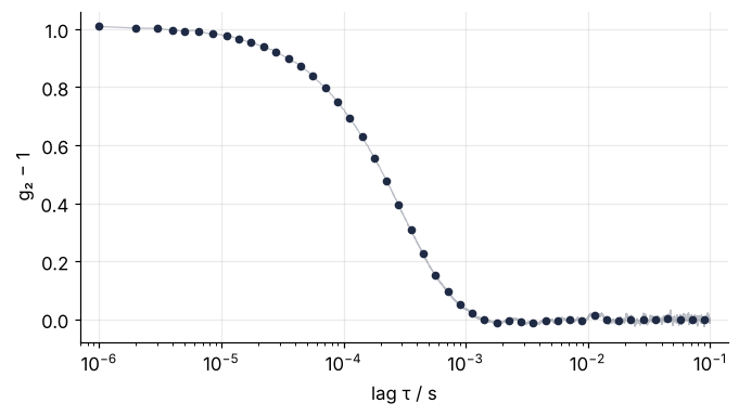
Intensity correlation g2 − 1 of the 100 nm sample against lag in s, log axis. Thin line: every lag, most of them crowded into the flat baseline past 1 ms. Dots: 47 averages over logarithmic bins, spread evenly across the decay.

47 bins from 1 µs to 90 ms
spread past 10 ms   single lags ±0.0089
                    new at each lag ±0.0010
                    bins ±0.0045, if the lags were independent ±0.0001

Rounding merges the first bins, so 47 remain. Past 10 ms, where \(g_2 - 1\) should be 0, the single lags scatter by ±0.009, and that scatter has two parts. The part that is new at every lag shows in the difference of neighbors, which carries the error of two lags: ±0.001 per lag. The rest is a slow wander that neighboring lags share, because 4.19 s hold only about 14,000 decay times. A bin averages the new part away but not what its lags have in common, so the bins still scatter by ±0.005, not the ±0.0001 that independent lags would give. Only a longer run shrinks the wander.

Step 4: Fit the Siegert relation and turn Γ into a diameter

For Gaussian light the intensity correlation follows from the field correlation by the Siegert relation \(g_2 = 1 + \beta|g_1|^2\), so

\[g_2(\tau) - 1 = \beta\,e^{-2\Gamma\tau}.\]

The intensity forgets twice as fast as the field, at 3,420 s⁻¹ for 100 nm. \(\beta\) is the coherence factor: 1 for a detector that sees one speckle, as here, and 0.3 to 0.9 on real instruments, whose pinhole sees several speckles at once and averages part of the flicker away. An instrument exports \(g_2 - 1\) on its own log lag grid, which np.loadtxt reads, so measured data starts here, with this curve_fit.

def siegert(tau, beta, gamma):
    return beta * np.exp(-2 * gamma * tau)

popt, pcov = curve_fit(siegert, tau, g2_binned - 1, p0=[1, 1000], bounds=(0, np.inf))
(beta, gamma), (beta_err, gamma_err) = popt, np.sqrt(np.diag(pcov))
print(f"β = {beta:.3f} ± {beta_err:.3f}")
print(f"Γ = {gamma:,.0f} ± {gamma_err:.0f} 1/s   (true {gamma_100:,.0f})")
print(f"d = {diameter(gamma) * 1e9:.1f} nm         (true 100)")

β = 1.012 ± 0.001
Γ = 1,675 ± 8 1/s   (true 1,711)
d = 102.2 nm         (true 100)

The fit finds \(\beta\) = 1.012 and \(\Gamma\) = 1,675 s⁻¹ against the true 1,711, so \(d\) = 102.2 nm for 100. The miss is 36 s⁻¹, more than four of the quoted errors: neighboring bins share the slow wander of Step 3, and pcov assumes independent errors. Its errors are a lower bound, and the miss is the statistical error of one 4 s measurement, not a bias, as nine samples show in Step 6.

Step 5: Mix two sizes: one exponential against cumulants

Take 50 nm and 200 nm spheres that each scatter half of the intensity. Their two independent fields add, each of variance 0.5, so \(g_1 = 0.5\,e^{-\Gamma_{50}\tau} + 0.5\,e^{-\Gamma_{200}\tau}\). Equal intensity is not equal numbers: in the Rayleigh limit intensity grows as \(d^6\), which would make it about 4,000 small particles per large one.

A fit that assumes no shape uses averages. \(g_1\) is the average of \(e^{-\Gamma\tau}\) over the decay rates in the sample. Write each rate as the mean \(\bar\Gamma\) plus a deviation and expand the exponential of the deviation: the first order averages to zero, the second leaves \(\ln g_1 = -\bar\Gamma\tau + \mu_2\tau^2/2\), with \(\mu_2\) the variance of the rates. Mean and variance are the first two cumulants of the rates, hence the method of cumulants. The Siegert relation squares \(g_1\), which doubles its logarithm:

\[\ln(g_2 - 1) = \ln\beta - 2\bar\Gamma\tau + \mu_2\tau^2 - \dots\]

That is a parabola in \(\tau\) for np.polyfit. I fit only bins where \(g_2 - 1\) is above a tenth of its first value, since further out the higher terms take over. The diameter of \(\bar\Gamma\) is the z-average, and \(\text{PDI} = \mu_2/\bar\Gamma^2\), the polydispersity index, is the relative spread of the rates, 0 for one size.

gamma_50, gamma_200 = diffusion(50e-9) * q**2, diffusion(200e-9) * q**2
field = np.sqrt(0.5) * scattered_field(gamma_50) + np.sqrt(0.5) * scattered_field(gamma_200)
tau_mix, g2_mix = log_bin(autocorrelate(photon_counts(field)))
y = g2_mix - 1

(beta_1, gamma_1), _ = curve_fit(siegert, tau_mix, y, p0=[1, 1000], bounds=(0, np.inf))

keep = y > y[0] / 10                                     # a choice; instruments differ here
c2, c1, c0 = np.polyfit(tau_mix[keep], np.log(y[keep]), 2)
gamma_bar, mu2 = -c1 / 2, c2

# what the cumulants should find for equal intensity fractions
gamma_true = 0.5 * (gamma_50 + gamma_200)
mu2_true = 0.5 * ((gamma_50 - gamma_true)**2 + (gamma_200 - gamma_true)**2)

fit_1 = siegert(tau_mix, beta_1, gamma_1)
fit_cumulants = np.exp(np.polyval([c2, c1, c0], tau_mix[keep]))
residual = y - fit_1

fig, (top, bottom) = plt.subplots(2, 1, figsize=(7, 4.6), sharex=True, height_ratios=[3, 2])
top.plot(tau_mix, y, "o", color=INK, ms=4)
top.plot(tau_mix, fit_1, color=ACCENT, lw=1.6)
top.plot(tau_mix[keep], fit_cumulants, color=SECOND)
top.set(ylabel="g₂ − 1")
bottom.axhline(0, color=MUTED, ls="--", lw=1)          # the misses, data minus fit
bottom.plot(tau_mix, residual, "o-", color=ACCENT, ms=4, lw=1.2)
bottom.plot(tau_mix[keep], y[keep] - fit_cumulants, "o-", color=SECOND, ms=4, lw=1.2)
bottom.text(3e-3, 0.02, "one exponential", color=ACCENT, va="center")
bottom.text(1.5e-6, -0.007, "cumulants", color=SECOND, va="center")
bottom.set(xscale="log", xlabel="lag τ / s", ylabel="data − fit", xlim=(7e-7, 0.14))
plt.show()

worst = np.argmax(np.abs(residual))
print(f"one exponential: d       = {diameter(gamma_1) * 1e9:5.1f} nm   "
      f"(largest miss {residual[worst]:+.3f} at {tau_mix[worst] * 1e3:.1f} ms)")
print(f"cumulants:       z-average = {diameter(gamma_bar) * 1e9:5.1f} nm   (expected {diameter(gamma_true) * 1e9:.1f})")
print(f"                 PDI     = {mu2 / gamma_bar**2:5.2f}      (expected {mu2_true / gamma_true**2:.2f}, {keep.sum()} bins)")

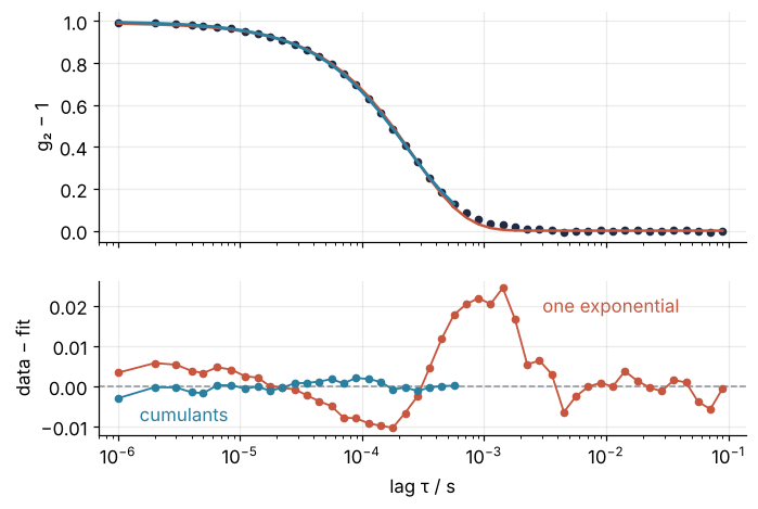
Top: g2 − 1 of a mixture of 50 and 200 nm spheres against lag in s, log axis, dots with the single-exponential and cumulant fits almost on top of them. Bottom: data minus fit. The single exponential misses in a wave that peaks at +0.024 near 1.4 ms; the cumulant residual stays near zero.

one exponential: d       =  88.2 nm   (largest miss +0.024 at 1.4 ms)
cumulants:       z-average =  81.4 nm   (expected 80.0)
                 PDI     =  0.23      (expected 0.36, 25 bins)

Since \(\Gamma\) is proportional to \(1/d\), averaging \(\Gamma\) averages \(1/d\): the z-average is a harmonic mean, 80 nm here, not the plain mean of 125 nm. The single exponential reads 88.2 nm. Its residual is a wave, worst at 1.4 ms with +0.024, where the 200 nm particles still correlate. Cumulants give a z-average of 81.4 nm against the expected 80 and a PDI of 0.23 against 0.36, biased low by the truncated range but well above the 0.1 instruments call monodisperse. The PDI flags the mixture that the single fit hides. Neither says that it holds 50 and 200 nm.

Step 6: Recover the size of nine samples from 20 to 500 nm

Steps 1 to 4 fit into one function, and one call per size gives the final figure.

def measure(d):
    tau, g2_binned = log_bin(autocorrelate(photon_counts(scattered_field(diffusion(d) * q**2))))
    popt, _ = curve_fit(siegert, tau, g2_binned - 1, p0=[1, 1000], bounds=(0, np.inf))
    return diameter(popt[1]), tau, g2_binned - 1, popt

sizes = [20, 30, 50, 70, 100, 150, 200, 300, 500]          # nm
results = {d: measure(d * 1e-9) for d in sizes}

fig, (top, bottom) = plt.subplots(2, 1, figsize=(7, 5.8), layout="constrained")
for d in (20, 100, 500):
    _, tau_d, y_d, popt = results[d]
    top.plot(tau_d, y_d, "o", color=INK, ms=4)
    top.plot(tau_d, siegert(tau_d, *popt), color=ACCENT)
    tau_half = np.log(2 * popt[0]) / (2 * popt[1])       # where the fit passes 0.5
    top.text(tau_half / 1.55, 0.5, f"{d} nm", color=INK, ha="center", va="center",
             rotation=-55, rotation_mode="anchor")        # parallel to the curve, left of it
top.set(xscale="log", xlabel="lag τ / s", ylabel="g₂ − 1", xlim=(7e-7, 0.14))

d_found = np.array([results[d][0] * 1e9 for d in sizes])
bottom.plot([15, 600], [15, 600], color=MUTED, ls="--", lw=1)
bottom.plot(sizes, d_found, "o", color=ACCENT, ms=6)
bottom.set(xscale="log", yscale="log", xlim=(15, 600), ylim=(15, 600),
           xticks=[20, 50, 100, 200, 500], yticks=[20, 50, 100, 200, 500],
           xticklabels=[20, 50, 100, 200, 500], yticklabels=[20, 50, 100, 200, 500],
           xlabel="true diameter / nm", ylabel="recovered diameter / nm")
bottom.minorticks_off()
plt.show()

print(" true    found   deviation")
for d, found in zip(sizes, d_found):
    print(f"{d:4d} nm {found:6.1f} nm   {100 * (found / d - 1):+5.1f} %")
print(f"spread of the deviations ±{100 * np.std(d_found / sizes - 1, ddof=1):.1f} %, "
      f"pcov in Step 4 claimed ±{100 * gamma_err / gamma:.1f} %")

Top: intensity correlation g2 − 1 against lag in s, log axis, for 20, 100, and 500 nm spheres, dots with their Siegert fits; the smaller the particle, the earlier the decay. Bottom: recovered diameter against true diameter, log axes, nine dots on the dashed diagonal.

 true    found   deviation
  20 nm   20.1 nm    +0.3 %
  30 nm   30.6 nm    +2.0 %
  50 nm   50.2 nm    +0.4 %
  70 nm   71.2 nm    +1.7 %
 100 nm  101.6 nm    +1.6 %
 150 nm  151.1 nm    +0.7 %
 200 nm  206.5 nm    +3.2 %
 300 nm  303.2 nm    +1.1 %
 500 nm  483.8 nm    -3.2 %
spread of the deviations ±1.8 %, pcov in Step 4 claimed ±0.5 %

Every size comes back within 3.5 %, with no trend from 20 to 500 nm, so the lag grid from 1 µs to 0.1 s covers the whole range: even the 20 nm decay, at \(2\Gamma\) = 17,000 s⁻¹, spans about 60 samples. The spread of the nine deviations, ±1.8 %, is the real error of one 4 s measurement, about four times the ±0.5 % that pcov claimed in Step 4.

Pitfalls

Fitting exp(−Γτ) to the intensity correlation. Every size comes out half the true one, and the 100 nm sample reads 51 nm. The cause is the Siegert relation: \(g_2 - 1\) decays at \(2\Gamma\), so a model with a single \(\Gamma\) in the exponent returns \(2\Gamma\), and Stokes-Einstein halves the diameter. Fit \(\beta e^{-2\Gamma\tau}\), or fit the rate as it comes and halve it before converting.

print(f"{diameter(2 * gamma) * 1e9:.1f} nm")      # what the wrong model reports for Step 4's sample

51.1 nm

Dust. A slow tail or a baseline above 1 at long lags, and a z-average that jumps from run to run. In the Rayleigh estimate the intensity grows as \(d^6\), so one 1 µm dust grain crossing the beam outshines \(20^6 \approx 6 \times 10^7\) particles of 50 nm, and while it is in the beam the correlation is mostly its own. Filter the sample through a 0.2 µm syringe filter, discard runs whose baseline at long lags is off, and look at the long lags before trusting the number.

Comparing DLS with electron microscopy. DLS reads several nanometers larger than TEM on the same particles. DLS measures the hydrodynamic diameter, the size of a sphere that diffuses equally fast, and that includes the solvation shell, ligands, and any polymer coat; it also depends on the viscosity and temperature you entered, and the viscosity of water drops by about 2 % per °C near 25 °C. Report the result as a hydrodynamic diameter with \(T\) and \(\eta\), and do not correct it to the TEM size. They measure different things.

Variations

Fluorescence correlation spectroscopy. Correlate the fluorescence counts from a confocal volume instead. The correlation then has amplitude \(1/N\), with \(N\) the number of molecules in the volume, and a 2D or 3D diffusion form in place of the exponential, so it gives the concentration as well as \(D\).
Several angles. Repeat the measurement at \(\theta\) from 30° to 150° and fit \(\Gamma\) against \(q^2\). The slope is \(D\), and an intercept that is not zero betrays a process other than diffusion.
Two populations. Replace the model by \(\beta\,(a\,e^{-\Gamma_a\tau} + (1-a)\,e^{-\Gamma_b\tau})^2\) in curve_fit. It finds two sizes, but rerun Step 5's mixture with fresh noise and the larger one moves by a factor of several around the true 200 nm, because rates only a factor of four apart are hard to separate in 4 s of counts.
A distribution of sizes. Fit \(g_1\) as a sum over a fixed grid of \(\Gamma\) values with scipy.optimize.nnls and a smoothness penalty, the idea behind Provencher's CONTIN (1982).

Cheat sheet

q = 4 * np.pi * n_medium / wavelength * np.sin(theta / 2)    # scattering vector, 1/m
d = kB * T * q**2 / (3 * np.pi * eta * gamma)                # Stokes-Einstein, Γ = D q²
F = np.fft.rfft(n_counts, 2 * N)                             # zero-pad: linear, not circular
g2 = np.fft.irfft(abs(F)**2)[:N] / (N - np.arange(N)) / n_counts.mean()**2
edges = np.unique(np.round(np.logspace(0, 5, 51)).astype(int))   # 10 bins per decade
siegert = lambda tau, beta, gamma: beta * np.exp(-2 * gamma * tau)   # g2 - 1 decays at 2Γ
popt, pcov = curve_fit(siegert, tau, g2_binned - 1, p0=[1, 1000], bounds=(0, np.inf))
keep = g2_binned - 1 > (g2_binned[0] - 1) / 10                # cumulants: only the first decade of the decay
c2, c1, c0 = np.polyfit(tau[keep], np.log(g2_binned[keep] - 1), 2)   # Γ̄ = -c1/2, PDI = c2/Γ̄²