Autocorrelation: how many independent hours a year of wind power holds

The question

A wind farm logs its capacity factor, the fraction of its rated power it delivers, once an hour for a year: 8,760 values between 0 and 1. The year's mean is 32.1 %, the hours scatter around it with a standard deviation of 0.3515, and the standard error of the mean comes out as 0.3515/√8760 = 0.0038, or 0.38 percentage points. Here are the first three weeks of that year, and below them the yearly means of 20 other years of the same farm:

Show code

Copy

import numpy as np
import matplotlib.pyplot as plt

plt.rcParams.update({
    "figure.figsize": (7, 3.6), "figure.dpi": 110,
    "axes.spines.top": False, "axes.spines.right": False,
    "axes.grid": True, "grid.alpha": 0.25,
    "font.size": 11, "lines.linewidth": 1.8,
})
INK, ACCENT, SECOND, MUTED = "#1f2a44", "#c8553d", "#2a7f9e", "#8a8f98"

# The farm is synthetic, so that every answer can be checked against a known truth.
N = 8760                                                   # hours in a year
TAU_WIND, LAM, DAILY, PEAK_HOUR = 48.0, 8.0, 0.25, 15     # h, m/s, relative swing, hour of the daily maximum
V_IN, V_RATED, V_OUT = 3.0, 12.0, 25.0                     # m/s
hour = np.arange(N)

def simulate(years, rng):
    phi = np.exp(-1 / TAU_WIND)
    uv = rng.standard_normal((2, years, N))                # two wind components, unit variance
    for t in range(1, N):
        uv[..., t] = phi * uv[..., t - 1] + np.sqrt(1 - phi**2) * uv[..., t]
    speed = LAM * np.sqrt((uv[0]**2 + uv[1]**2) / 2)       # Weibull, shape 2, scale LAM
    speed *= 1 + DAILY * np.cos(2 * np.pi * (hour - PEAK_HOUR) / 24)
    # a cubic power curve between cut-in and rated speed, a simplification of a real turbine's
    cf = np.clip((speed**3 - V_IN**3) / (V_RATED**3 - V_IN**3), 0, 1)
    cf[speed >= V_OUT] = 0
    return cf, speed

x = simulate(1, np.random.default_rng(13))[0][0]           # the year
others = simulate(1000, np.random.default_rng(2026))[0]    # the same farm, 1,000 more years

def longest_run(mask):
    """Length of the longest stretch of consecutive True values, in samples."""
    edges = np.diff(np.concatenate([[0], mask.astype(int), [0]]))
    return np.max(np.flatnonzero(edges == -1) - np.flatnonzero(edges == 1))

naive = x.std() / np.sqrt(N)
means20 = 100 * others[:20].mean(axis=1)
print(f"this year:      mean {100 * x.mean():5.2f} %   sd {x.std():.4f}   naive standard error {100 * naive:.2f} points")
print(f"longest calm (below 5 %): {longest_run(x < 0.05)} h   longest at full power: {longest_run(x >= 1)} h")
print(f"20 other years: means from {means20.min():.1f} to {means20.max():.1f} %, sd {means20.std(ddof=1):.2f} points")

fig, (ax1, ax2) = plt.subplots(2, 1, figsize=(7, 4.6), height_ratios=[2, 1], layout="constrained")
weeks3 = hour < 21 * 24
ax1.plot(hour[weeks3] / 24, x[weeks3], color=INK, lw=1)
ax1.set(xlabel="time / days", ylabel="capacity factor", xlim=(0, 21), ylim=(-0.03, 1.05), xticks=range(0, 22, 3))
offsets = np.tile([0.0, 0.12, 0.24, 0.06, 0.18], 4)        # fixed heights, so dots do not hide each other
ax2.plot(means20, 1 + offsets, "o", color=INK, ms=5)
m = 100 * x.mean()
ax2.plot([m - 200 * naive, m + 200 * naive], [0.2, 0.2], color=MUTED, lw=5, solid_capstyle="butt")
ax2.plot(m, 0.2, "o", color=INK, ms=7, mec="white", mew=1.5)
ax2.text(m - 200 * naive - 0.15, 0.2, "± 2 naive standard errors", color=MUTED, ha="right", va="center")
ax2.set(xlabel="yearly mean capacity factor / %", ylim=(-0.2, 1.5), yticks=[0.2, 1.12],
        yticklabels=["this year", "20 others"])
ax2.grid(axis="y", visible=False)
plt.show()

this year:      mean 32.06 %   sd 0.3515   naive standard error 0.38 points
longest calm (below 5 %): 57 h   longest at full power: 44 h
20 other years: means from 26.6 to 33.3 %, sd 2.04 points

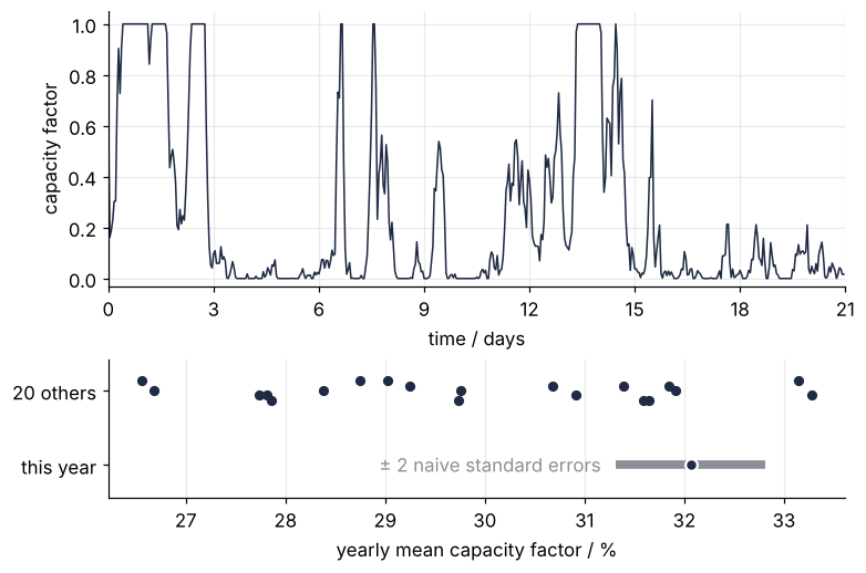
The data are synthetic, with a known truth to check against. The farm has a daily cycle that is the same on every day of every year, a fixed pattern of this synthetic farm and not weather. I picked seed 13 for the analyzed year from a scan of 60 seeds because it is a typical year, and the comparison years come from a generator of their own; Formalization shows how far 200 other years scatter, so nothing rests on the pick.

Some things are obvious. The output swings between 0 and 1 within a day. Calm spells and windy spells last for days: the longest stretch below 5 % runs 57 h, the longest at full power 44 h. The output tends to rise in the afternoon. And the standard error says the yearly mean is known to better than half a point.

Less obvious: the other years disagree. Their means run from 26.6 to 33.3 % and scatter with a standard deviation of 2.04 points, more than five times the standard error. The formula assumed 8,760 independent hours, and a windy hour is usually followed by another windy hour. How much does an hour remember of the hours before it, how long does that memory last, and how many independent hours does a year really hold?

The idea: slide the series along a copy of itself

Standardize the series first: subtract the mean and divide by the standard deviation, so that a windy hour is a positive number, a calm hour a negative one, and a typical deviation has size 1. Shift a copy by k hours, multiply the two hour by hour, and average the product over the hours where they overlap. Where windy hours meet windy hours, or calm meets calm, the product is positive. If an hour still remembers the weather k hours earlier, such meetings dominate and the average is clearly positive. Once the shift is longer than the memory, the signs meet at random and the average is near zero. If you know the Fourier transform, this is its probe, with the series as its own probe.

The average product of two deviations is called the covariance of the two series, and for standardized series it is their correlation, a number between −1 and 1. Here the two series are one series and its shifted copy, hence autocorrelation, and as a function of k it is the autocorrelation function.

z = (x - x.mean()) / x.std()

def overlap_average(z, k):
    """Average product of z and its copy shifted by k samples, over the overlap."""
    return np.mean(z[:len(z) - k] * z[k:])         # len(z) - k, not -k: k = 0 must keep the whole series

print(f"k = 0: {overlap_average(z, 0):.3f}")

k = 0: 1.000

Here is the slide at three shifts, over five days of the year:

Show code

Copy

window = (hour >= 240) & (hour < 360)                      # days 10 to 15
fig, axes = plt.subplots(3, 1, figsize=(7, 6.3), sharex=True, sharey=True, layout="constrained")
for ax, k in zip(axes, [3, 12, 24]):
    copy = np.roll(z, k)                                   # copy[t] = z[t - k]; the window starts well past k
    ax.plot(hour[window], z[window], color=INK, label="series")
    ax.plot(hour[window], copy[window], color=SECOND, lw=1.2, label="shifted copy")
    ax.fill_between(hour[window], 0, (z * copy)[window], color=ACCENT, alpha=0.35, lw=0, label="product")
    ax.text(0.01, 0.95, f"lag k = {k} h   average = {overlap_average(z, k):+.2f}",
            transform=ax.transAxes, ha="left", va="top")
    ax.set(ylabel="deviation / sd", ylim=(-2.2, 4.4))
fig.legend(*axes[0].get_legend_handles_labels(), frameon=False, loc="outside upper center", ncol=3)
axes[-1].set(xlabel="time / h", xlim=(240, 360))
plt.show()

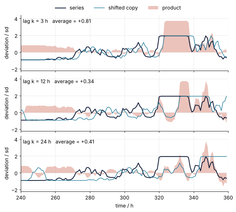
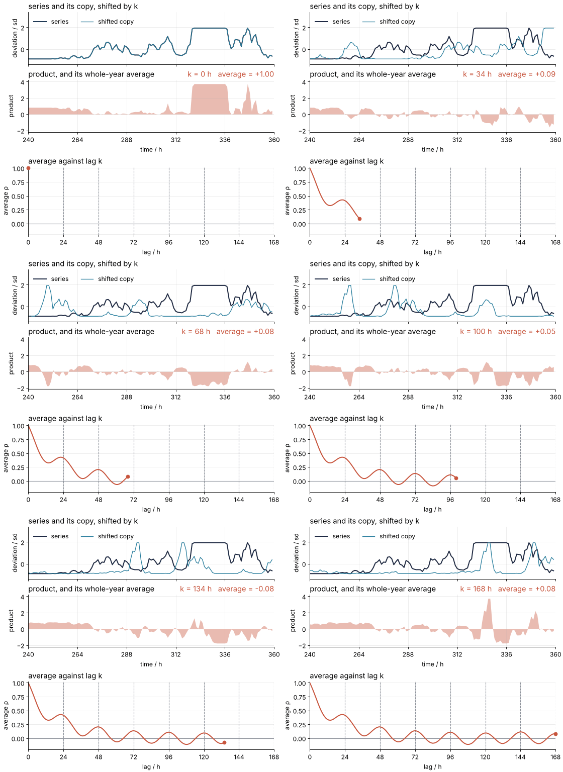
At a shift of 3 h the copy nearly covers the series, the product is positive almost everywhere, and the whole-year average is 0.81. At 12 h it has dropped to 0.34. At 24 h it is 0.41, higher again: a day later the series resembles itself more than half a day later. Watch the copy slide and the function being traced out:

"""ACF sweep: the autocorrelation function as the average product of a series and its shifted copy.

Renders ../../assets/acf-sweep.gif from the synthetic wind-power year of py-autocorrelation
(same generator, same seed). Run it from any directory:

    python scene.py
"""
from pathlib import Path

import numpy as np
import matplotlib.pyplot as plt
from matplotlib.animation import FuncAnimation, PillowWriter
from PIL import Image

OUT = Path(__file__).resolve().parents[2] / "assets" / "acf-sweep.gif"
INK, ACCENT, SECOND, MUTED = "#1f2a44", "#c8553d", "#2a7f9e", "#8a8f98"
plt.rcParams.update({"axes.spines.top": False, "axes.spines.right": False,
                     "axes.grid": True, "grid.alpha": 0.25, "font.size": 11})

# ---- data: the year of the tutorial, exactly as its setup cell draws it
N = 8760
TAU_WIND, LAM, DAILY, PEAK_HOUR = 48.0, 8.0, 0.25, 15
V_IN, V_RATED, V_OUT = 3.0, 12.0, 25.0
hour = np.arange(N)

def simulate(years, rng):
    phi = np.exp(-1 / TAU_WIND)
    uv = rng.standard_normal((2, years, N))
    for t in range(1, N):
        uv[..., t] = phi * uv[..., t - 1] + np.sqrt(1 - phi**2) * uv[..., t]
    speed = LAM * np.sqrt((uv[0]**2 + uv[1]**2) / 2)
    speed *= 1 + DAILY * np.cos(2 * np.pi * (hour - PEAK_HOUR) / 24)
    cf = np.clip((speed**3 - V_IN**3) / (V_RATED**3 - V_IN**3), 0, 1)
    cf[speed >= V_OUT] = 0
    return cf, speed

x = simulate(1, np.random.default_rng(13))[0][0]
z = (x - x.mean()) / x.std()

def overlap_average(z, k):
    return np.mean(z[:len(z) - k] * z[k:])

K_MAX = 168
lags = np.arange(K_MAX + 1)
rho = np.array([overlap_average(z, k) for k in lags])
window = (hour >= 240) & (hour < 360)                                # the five days of the static figure
tw = hour[window]

# the frame values: lags 0 to 168 in steps of 2, holding on the bump at 24 h and at the end
frames = list(range(0, 25, 2)) + [24] * 8 + list(range(26, K_MAX + 1, 2)) + [K_MAX] * 10

# ---- figure, drawn once
fig, (ax1, ax2, ax3) = plt.subplots(3, 1, figsize=(7, 6.4), dpi=80, height_ratios=[1, 1, 1.3],
                                    layout="constrained")
ax1.plot(tw, z[window], color=INK, lw=1.8, label="series")
(copy_line,) = ax1.plot([], [], color=SECOND, lw=1.2, label="shifted copy")
ax1.legend(frameon=False, loc="upper left", ncol=2)
product_fill = ax2.fill_between(tw, 0, 0, color=ACCENT, alpha=0.4, lw=0)
avg_text = ax2.set_title(" ", loc="right", color=ACCENT)                    # the readout, beside the panel title
for day in range(24, K_MAX + 1, 24):
    ax3.axvline(day, color=MUTED, lw=1, ls="--")
ax3.axhline(0, color=MUTED, lw=1)
(trace,) = ax3.plot([], [], color=ACCENT, lw=1.8)
(dot,) = ax3.plot([], [], "o", color=ACCENT, ms=6, clip_on=False, zorder=3)   # whole at k = 0 and k = 168
for ax in (ax1, ax2):
    ax.set(xlim=(240, 360), xticks=range(240, 361, 24))
ax1.set(ylabel="deviation / sd", ylim=(-1.4, 3.4))
ax1.tick_params(labelbottom=False)                                   # time is labeled once, below
ax2.set(ylabel="product", xlabel="time / h", ylim=(-2.2, 4.2))
ax3.set(ylabel="average ρ", xlabel="lag / h", xlim=(0, K_MAX), ylim=(-0.2, 1.02),
        xticks=range(0, K_MAX + 1, 24))
ax1.set_title("series and its copy, shifted by k", loc="left")
ax2.set_title("product, and its whole-year average", loc="left")
ax3.set_title("average against lag k", loc="left")

# ---- one frame: a function of the lag alone
def update(k):
    copy = np.roll(z, k)[window]                                     # copy[t] = z[t - k]
    copy_line.set_data(tw, copy)
    product_fill.set_data(tw, 0, z[window] * copy)
    avg_text.set_text(f"k = {k} h   average = {rho[k]:+.2f}")
    trace.set_data(lags[:k + 1], rho[:k + 1])
    dot.set_data([k], [rho[k]])

# ---- render, and read back what was written
OUT.parent.mkdir(exist_ok=True)
FuncAnimation(fig, update, frames=frames).save(OUT, writer=PillowWriter(fps=12))
plt.close(fig)
with Image.open(OUT) as im:
    delay = im.info["duration"]
    print(f"{OUT.name}: {im.width} x {im.height} px, {im.n_frames} frames at {delay} ms, "
          f"{im.n_frames * delay / 1000:.1f} s, {OUT.stat().st_size / 1024:,.0f} kB")

The same overlap_average, in a loop over every shift from 0 to 240 h:

Show code

Copy

lags = np.arange(241)
rho = np.array([overlap_average(z, k) for k in lags])
dip = np.argmin(rho[:20])
bump = 15 + np.argmax(rho[15:30])
print(f"rho at 1 h: {rho[1]:.2f}   dip {rho[dip]:.2f} at {dip} h   bump {rho[bump]:.2f} at {bump} h   "
      f"first zero at {np.argmax(rho < 0)} h   rho at 36 h: {rho[36]:.2f}")

fig, ax = plt.subplots()
for day in range(24, 241, 24):
    ax.axvline(day, color=MUTED, lw=1, ls="--")
ax.axhline(0, color=MUTED, lw=1)
ax.plot(lags, rho, color=ACCENT)
ax.annotate(f"bump {rho[bump]:.2f} at {bump} h", (bump, rho[bump]), xytext=(40, 0.62), color=ACCENT,
            bbox=dict(fc="white", ec="none", pad=1.5), arrowprops=dict(arrowstyle="-", color=ACCENT, lw=1))
ax.set(xlabel="lag / h", ylabel="autocorrelation ρ", xlim=(0, 240), ylim=(-0.25, 1.02),
       xticks=range(0, 241, 48))
plt.show()

rho at 1 h: 0.94   dip 0.32 at 14 h   bump 0.43 at 22 h   first zero at 57 h   rho at 36 h: 0.05

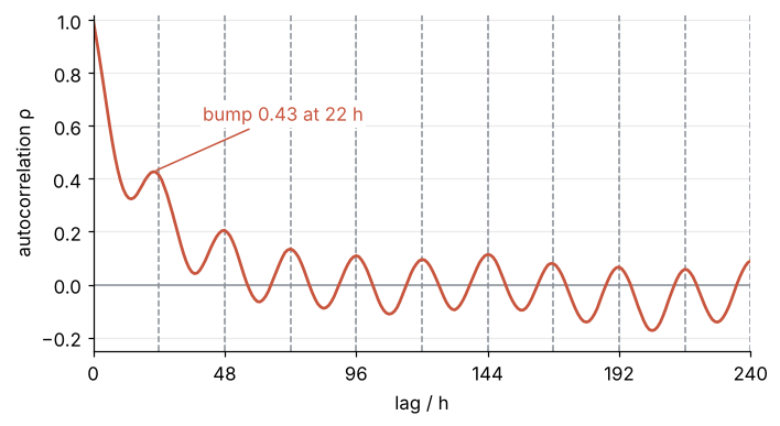
The function starts at 1, because every series matches itself, and is still 0.94 one hour later. It dips to 0.32 at 14 h, climbs back to a bump of 0.43 at 22 h, and first crosses zero at 57 h. Then it does not settle.

The daily cycle, and a ripple that never fades

A daily cycle matches itself every 24 h: shift the series by a day and 15:00 meets 15:00. That is the bump, and the dip is the afternoon meeting the night. The weather part is still falling underneath, which pulls the bump back from 24 h to 22 h and pushes the dip out from 12 h to 14 h. Average each clock hour over the 365 days and you get the year's mean daily profile:

profile = x.reshape(365, 24).mean(axis=0)                  # one value per clock hour
print(f"mean daily profile: {profile.min():.2f} at {np.argmin(profile):02d}:00, "
      f"{profile.max():.2f} at {np.argmax(profile):02d}:00")
print(f"variance of the profile: {100 * profile.var() / x.var():.0f} % of the variance of the hourly series")

mean daily profile: 0.16 at 03:00, 0.48 at 15:00
variance of the profile: 11 % of the variance of the hourly series

The profile runs from 0.16 at 03:00 to 0.48 at 15:00, and its variance is 11 % of that of the hourly series: about a tenth of the hour-to-hour swings is the clock, the rest is weather.

The function above was computed as if the statistics of the series were the same at every hour, so that ρ depends only on the shift and not on where in the year you start. That property is called stationarity. The daily cycle breaks it mildly: the expected output depends on the time of day, but the clock holds only 11 % of the variance. A trend would break it too, and you subtract it first, as with the cycle below.

The ripple is the trace the cycle leaves. A fixed periodic pattern never decays, so from the third day on the function swings between about +0.1 at whole days and −0.1 at half days, out to 240 h and beyond. The weather part fades within two to three days: ρ is 0.05 at 36 h, and what is left after that is ripple and noise.

For the error of a yearly mean the ripple costs nothing here, for two reasons. The cycle is the same in every year, so it cannot make one year's mean differ from another's. And a year holds 365 whole days, so the cycle averages out of the mean exactly. Both are properties of this synthetic farm, not of periodic signals in general. The general test is to remove the cycle and compute again, by subtracting the mean daily profile from every day:

resid = x - np.tile(profile, 365)                          # the year without its mean daily cycle
z_resid = (resid - resid.mean()) / resid.std()
print(f"rho at 120 h: {overlap_average(z, 120):+.3f} with the daily cycle, "
      f"{overlap_average(z_resid, 120):+.3f} without it")

rho at 120 h: +0.095 with the daily cycle, -0.013 without it

At 120 h, five whole days, ρ falls from 0.09 to −0.01, and the ripple is gone. A mean profile removes only a cycle that repeats unchanged. One that changes from day to day or year to year, or a record that does not hold whole periods, needs seasonal decomposition, the subject of a planned tutorial, to remove it before you compute the autocorrelation of what is left. See it in code repeats the error with the cycle removed, once the error is defined.

Formalization

For a series \(x_1, \dots, x_N\) with mean \(\bar x\), the autocovariance at lag \(k\) and the autocorrelation are

\(c_k\) is the overlap average of the previous section, divided by \(N\) instead of by the \(N - k\) pairs in the overlap, and \(c_0\) is the variance; the reason for \(N\) comes below.

def acf(x, max_lag):
    d = x - x.mean()
    c = np.array([d[:len(x) - k] @ d[k:] for k in range(max_lag + 1)]) / len(x)
    return c / c[0]

r = acf(x, N - 1)                                          # every lag of the year

Two values show why this function sets the error of a mean. Square the sum of two deviations, \((a + b)^2 = a^2 + b^2 + 2ab\), and average it, and you get \(\operatorname{Var}(X + Y) = \operatorname{Var}(X) + \operatorname{Var}(Y) + 2\operatorname{Cov}(X, Y)\). Rule 1 of the standard error is the case \(\operatorname{Cov} = 0\). Two neighboring hours of the year have \(\operatorname{Cov} = \sigma^2\rho_1\), so their sum has \(1 + \rho_1 = 1.94\) times the variance rule 1 gives:

pair_sums = x[:-1] + x[1:]                                 # the year's 8,759 neighboring pairs
print(f"Var(x_t + x_t+1) / 2 sigma^2 = {pair_sums.var() / (2 * x.var()):.2f}   1 + rho_1 = {1 + r[1]:.2f}")

Var(x_t + x_t+1) / 2 sigma^2 = 1.94   1 + rho_1 = 1.94

Square the sum of \(N\) values instead: of the \(N^2\) terms, \(N\) are variances, and the \(2(N - k)\) terms whose two hours are \(k\) apart contribute \(\sigma^2\rho_k\) each. Dividing by \(N^2\) gives the variance of the mean,

where the approximation holds when the memory is short against the record. \(\tau\) is the correlation time and \(N_\text{eff} = N/\tau\) the effective sample size, the number of independent values that would give as good a mean. \(\tau\) counts samples, here hours, and \(N\) must count the same samples. Some books call half of this the integrated correlation time; this page follows emcee.

Divide by N, and the full sum is zero. Divided by \(N - k\), the function rests on a handful of pairs at the far lags and swings between −1.08 and +0.45 over the last 60. Dividing by \(N\) damps them, at the price of pulling \(\hat\rho_k\) low by \((N - k)/N\), under 2 % over the first week of lags. Summed over every lag, though, \(1 + 2\sum_k \hat\rho_k\) is exactly zero. The deviations from the sample mean add up to zero, so the square of their sum is zero, and the expansion above, over all \(N\) deviations, says \(N(c_0 + 2\sum_k c_k) = 0\).

d = x - x.mean()
tail = np.array([d[:N - k] @ d[k:] / (N - k) for k in range(N - 60, N)]) / d.var()
print(f"divided by N - k, lags {N - 60} to {N - 1}: from {tail.min():+.2f} to {tail.max():+.2f}")
print(f"divided by N, 1 + 2 sum over every lag: {1 + 2 * r[1:].sum():.1e}")

divided by N - k, lags 8700 to 8759: from -1.08 to +0.45
divided by N, 1 + 2 sum over every lag: 1.2e-13

A \(\tau\) of zero would claim infinitely many independent hours, so the sum has to be cut.

Cut where the sum has settled. Cut at lag \(M\), the sum gives \(\tau(M)\). Each added lag brings in more of the true memory, so the part still left out shrinks as \(M\) grows, and more estimation noise, which grows with \(M\). The window must be several \(\tau\) long, and \(\tau\) is not known in advance, so the rule ties one to the other: take the smallest \(M\) with \(M \ge c\,\tau(M)\), here with \(c = 5\).

def tau_window(r, c=5):
    taus = 1 + 2 * np.cumsum(r[1:])                        # tau(M) for M = 1, 2, ...
    M = np.arange(1, len(r))
    i = np.argmax(M >= c * taus)                           # the smallest M with M >= c tau(M)
    return M[i], taus[i]

M, tau = tau_window(r)
print(f"window M = {M} h, tau = {tau:.1f} h")

window M = 178 h, tau = 35.2 h

The truth to check \(\tau\) against comes from the 1,000 other years. The standard deviation of their yearly means, 2.21 points, is the true standard error, and solving \(\operatorname{Var}(\bar x) \approx \sigma^2\tau/N\) for \(\tau\) turns it into 36.5 h:

Show code

Copy

yearly = others.mean(axis=1)
tau_true = N * yearly.var(ddof=1) / others.var()           # the tau that reproduces the spread of 1,000 yearly means
print(f"truth from 1,000 years: tau = {tau_true:.1f} h")

taus = 1 + 2 * np.cumsum(r[1:])
Ms = np.arange(1, N)
fig, ax = plt.subplots()
ax.plot(Ms, Ms / 5, color=MUTED, lw=1, ls="--")
ax.axhline(tau_true, color=SECOND, lw=1, ls="--")
ax.plot(Ms, taus, color=ACCENT)
ax.plot(M, tau, "o", color=ACCENT, ms=7, mec="white", mew=1.5, zorder=3)
ax.annotate(f"M = {M} h\nτ = {tau:.1f} h", (M, tau), xytext=(M, 12), color=ACCENT, ha="center", va="top",
            arrowprops=dict(arrowstyle="-", color=ACCENT, lw=1, shrinkB=5))
ax.text(1.2, tau_true + 2, f"truth {tau_true:.1f} h", color=SECOND, va="bottom")
ax.text(22, 6.5, "τ = M/5", color=MUTED, ha="right")
ax.set(xscale="log", xlabel="cutoff M / h", ylabel="τ(M) / h", xlim=(1, N), ylim=(-30, 60),
       xticks=[1, 10, 100, 1000], xticklabels=["1", "10", "100", "1,000"])
plt.show()

truth from 1,000 years: tau = 36.5 h

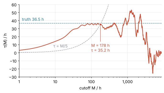
\(\tau(M)\) climbs for two days, settles near 35 h, and meets the line \(M/5\) at 178 h. Beyond about 1,000 h it wanders and falls to zero.

Over 200 simulated years, the choice of \(c\) is a trade:

r200 = [acf(y, 2000) for y in others[:200]]
print(" c   median tau   16th to 84th percentile")
for c in [1, 3, 5, 20]:
    t = np.array([tau_window(ry, c)[1] for ry in r200])
    lo, med, hi = np.percentile(t, [16, 50, 84])
    print(f"{c:2d}   {med:6.1f} h     {lo:5.1f} to {hi:5.1f} h  (±{100 * (hi - lo) / 2 / med:.0f} %)")

t_month = np.array([tau_window(acf(y[:720], 719))[1] for y in others[:200]])
print(f"\nfirst 720 h of each year: median tau {np.median(t_month):.1f} h, "
      f"{100 * np.mean(720 < 50 * t_month):.0f} % shorter than 50 tau")

 c   median tau   16th to 84th percentile
 1     23.9 h      19.6 to  28.7 h  (±19 %)
 3     34.8 h      28.6 to  43.3 h  (±21 %)
 5     35.2 h      26.7 to  44.9 h  (±26 %)
20     29.0 h      18.8 to  42.6 h  (±41 %)

first 720 h of each year: median tau 21.1 h, 82 % shorter than 50 tau

With \(c = 1\) the median is 24 h, a third too low. With \(c = 5\) it is 35.2 h, spread by ±26 % (26.7 to 44.9 h, the 16th to 84th percentile, ±1 standard deviation for a normal spread), and with \(c = 20\) by ±41 %. Keep \(c = 5\), the default of emcee.autocorr.integrated_time: 3 does as well here, and the default keeps \(\tau\) comparable across papers. ±26 % on \(\tau\) is ±13 % on the error, which goes as \(\sqrt\tau\).

The rule always returns a number, so a short record shows up only as a \(\tau\) that is too low. The first month of each year, about 20 \(\tau\), gives a median of 21 h against the true 36.5 h, because the deviations are measured from the month's own mean, which follows the slow swings. emcee refuses records under 50 \(\tau\); this year is 249 \(\tau\). Below about 50, read \(\tau\) as a lower bound.

The effective sample size, checked by blocks. With \(\tau = 35.2\) h the year holds 249 independent hours, and the error is 2.23 points instead of 0.38:

N_eff = N / tau
se = x.std() / np.sqrt(N_eff)
print(f"N_eff = {N_eff:.0f}   corrected standard error {100 * se:.2f} points   naive {100 * naive:.2f} points")

N_eff = 249   corrected standard error 2.23 points   naive 0.38 points

A check that needs no \(\rho\): cut the year into blocks of \(B\) hours and treat the block means as the samples.

Show code

Copy

blocks = np.array([1, 3, 6, 12, 24, 48, 96, 120, 168, 240, 336, 730])
se_blocks = []
for B in blocks:
    bm = x[:N // B * B].reshape(-1, B).mean(axis=1)        # drop the incomplete last block
    se_blocks.append(bm.std(ddof=1) / np.sqrt(bm.size))
se_blocks = 100 * np.array(se_blocks)
print("B / h:   " + "  ".join(f"{B:4d}" for B in blocks))
print("points:  " + "  ".join(f"{s:4.2f}" for s in se_blocks))

se_true = 100 * yearly.std(ddof=1)
fig, ax = plt.subplots()
ax.axhline(100 * naive, color=MUTED, lw=1, ls="--")
ax.axhline(100 * se, color=ACCENT, lw=1.6)
ax.axhline(se_true, color=SECOND, lw=1, ls="--")
ax.plot(blocks, se_blocks, "o", color=INK, ms=6)
ax.text(780, 100 * naive + 0.08, f"naive {100 * naive:.2f}", color=MUTED, ha="right", va="bottom")
ax.text(1.1, 100 * se + 0.08, f"corrected {100 * se:.2f}", color=ACCENT, va="bottom")
ax.text(1.1, se_true - 0.08, f"truth {se_true:.2f}", color=SECOND, va="top")
ax.set(xscale="log", xlabel="block length / h", ylabel="standard error / points",
       xlim=(0.9, 800), ylim=(0, 2.6), xticks=[1, 6, 24, 168, 730], xticklabels=["1", "6", "24", "168", "730"])
ax.minorticks_off()
plt.show()

B / h:      1     3     6    12    24    48    96   120   168   240   336   730
points:  0.38  0.63  0.86  1.13  1.43  1.73  1.99  2.07  2.09  2.14  2.00  1.77

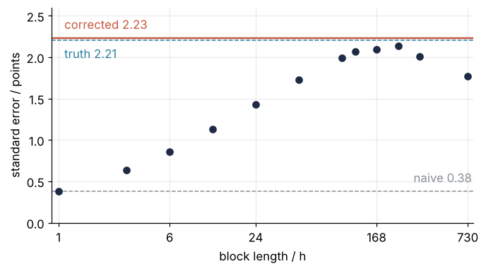
The error rises from the naive 0.38 points and levels off at 2.07 to 2.14 points for blocks of 5 to 10 days, several \(\tau\) long and so nearly independent. At a month only 12 blocks remain, and the estimate turns noisy.

See it in code

NumPy computes all the overlap sums at once with np.correlate. The cell checks it against acf, applies the window, and sets the year's answer beside every check this page has, including the truth from 1,000 simulated years and how often each error bar contains the long-run mean:

def correlation_time(x):
    d = x - x.mean()
    r = np.correlate(d, d, "full")[len(x) - 1:]            # "full" holds lags -(N - 1) to N - 1; keep 0 on
    return tau_window(r / r[0])[1]

d = x - x.mean()
r_np = np.correlate(d, d, "full")[N - 1:]
print(f"np.correlate against acf: largest difference {np.max(np.abs(r_np / r_np[0] - r)):.1e}\n")

tau_resid = correlation_time(resid)
rows = [("naive, independent hours", "", 100 * naive),
        ("corrected, this year", f"{tau:4.1f}", 100 * se),
        ("corrected, daily cycle removed", f"{tau_resid:4.1f}", 100 * resid.std() * np.sqrt(tau_resid / N)),
        ("block means, B = 168 h", "", se_blocks[list(blocks).index(168)]),
        ("truth, sd of 1,000 yearly means", f"{tau_true:4.1f}", se_true)]
print(f"{'':32s} tau / h   standard error / points")
for name, t, s in rows:
    print(f"{name:32s} {t:>6s}    {s:5.2f}")
print(f"\ntruth: N_eff = {N / tau_true:.0f}, standard error {se_true / (100 * naive):.1f} times the naive one")

mu = 100 * others.mean()                                   # the long-run mean of the farm
hits_naive = hits_corr = 0
for y in others[:200]:
    m, s = 100 * y.mean(), 100 * y.std() / np.sqrt(N)
    hits_naive += abs(m - mu) < 2 * s
    hits_corr += abs(m - mu) < 2 * s * np.sqrt(correlation_time(y))
print(f"mean ± 2 errors contains the long-run mean: naive in {hits_naive} of 200 years, corrected in {hits_corr}")
print(f"N_eff from rho_1 alone, N (1 - rho_1) / (1 + rho_1): {N * (1 - r[1]) / (1 + r[1]):.0f}")

np.correlate against acf: largest difference 1.1e-16

                                 tau / h   standard error / points
naive, independent hours                    0.38
corrected, this year               35.2     2.23
corrected, daily cycle removed     38.0     2.19
block means, B = 168 h                      2.09
truth, sd of 1,000 yearly means    36.5     2.21

truth: N_eff = 240, standard error 5.9 times the naive one
mean ± 2 errors contains the long-run mean: naive in 59 of 200 years, corrected in 192
N_eff from rho_1 alone, N (1 - rho_1) / (1 + rho_1): 268

The year's \(\tau\) of 35.2 h is within 4 % of the 36.5 h of 1,000 years, well inside the ±26 % one year can promise, and its corrected error is within 1 % of the true 2.21 points, where the naive one is off by a factor of 5.9. An interval of mean ± 2 naive errors contains the long-run mean in 59 of 200 simulated years, the corrected one in 192. With the daily cycle removed, \(\tau\) rises to 38.0 h, but the variance falls by the cycle's 11 %, and the error follows \(\sigma^2\tau\), not \(\tau\) alone: 2.19 points, so the cycle cost nothing. The answer for this record is 2.23 points, and the other rows are checks on it.

Both acf and np.correlate cost about \(N^2\) operations, which is instant for a year of hours. For records of millions of points, libraries compute the same function through the Fourier transform in \(N \log N\), as statsmodels' acf(fft=True) and emcee do.

Where it shows up

• Statistics and MCMC. A Markov chain's samples are correlated by construction, because each step starts from the last. emcee's get_autocorr_time is this \(\tau\) with the same window, and MCMC with emcee counts its independent samples as walkers times steps divided by \(\tau\).
• Molecular dynamics. The Green-Kubo relation gives the diffusion coefficient as \(D = \frac13 \int_0^\infty C_v(t)\,dt\), where \(C_v(t)\) is \(\mathbf v(0)\cdot\mathbf v(t)\) averaged over particles and starting times, the velocity autocorrelation. Viscosity comes the same way from the autocorrelation of the shear stress.
• Fluid dynamics and engineering. A hot-wire anemometer's velocity record gives the integral time scale of a turbulent flow, the integral of \(\rho\) over positive lags, about half the \(\tau\) of this page. Taylor's frozen-turbulence hypothesis multiplies it by the mean speed and turns it into the integral length scale of the eddies.
• Climate. A temperature anomaly record is often modeled as red noise, where each value keeps a fraction \(\rho_1\) of the previous one and adds fresh noise. Then \(\rho_k = \rho_1^k\) and \(\tau = (1 + \rho_1)/(1 - \rho_1)\), so the significance of a trend uses \(N_\text{eff} = N(1 - \rho_1)/(1 + \rho_1)\), which for this year of wind would give 268 against the window's 249.
• Lab measurements. Repeated readings of a reference standard drift, and past some number of readings averaging stops helping: the shared offset of the standard error, in slow motion. Clock and oscillator makers measure where that happens with the Allan variance.
• Neuroscience. The autocorrelogram of a spike train shows a dip at short lags, where the refractory period forbids a second spike. Bursting or rhythmic firing shows up as side peaks, like the daily bump here.

In every case the data hold as many independent samples as the record is long divided by the correlation time, and that number, not the count of points, goes under the square root.

Further reading

• numpy.correlate for the function and its mode argument.
• statsmodels.tsa.stattools.acf, the library route, with fft=True for long records and confidence bands for \(\hat\rho_k\).
• The emcee documentation on autocorrelation analysis, for the window rule, which emcee takes from Sokal's lecture notes Monte Carlo Methods in Statistical Mechanics: Foundations and New Algorithms, and its behavior on short chains.
• Chris Chatfield, The Analysis of Time Series: An Introduction (6th ed., Chapman & Hall/CRC, 2003), for the autocorrelation function, stationarity, and removing trends and cycles.
• Related tutorials on this site: The standard error of the mean: why four times the data halves the error, the rule this page corrects; MCMC with emcee: the half-life and background of a counting experiment, where \(\tau\) decides how much of a chain to keep; The Fourier transform: asking a signal how much of each frequency it contains, the probe idea; Matplotlib animation with FuncAnimation: a probe sweep as a small GIF, how the animation was built; The Kalman filter: a battery's charge from a drifting current and noisy voltage, another way to treat a series whose values remember each other; planned: autoregressive models, seasonal decomposition, and the same tutorial in Julia.
• Download the notebook. It was executed with the library versions in the header.