Find peaks with scipy.signal.find_peaks: heartbeats in a noisy pulse signal

The problem: a heart rate from a noisy pulse signal

A pulse oximeter clipped to a fingertip records a photoplethysmogram, or PPG: the light absorbed by the blood in the fingertip, which swells once per beat. Here are 30 s of it at 100 samples per second, and we want the heart rate. Every beat is a peak, and scipy.signal.find_peaks is the function that finds peaks. Two things get in its way. About 0.28 s after each beat comes a smaller second bump, the dicrotic wave, and the whole record drifts up and down with breathing and finger pressure by more than the height of a beat. The plan is to find the beats, take the median time between them, and turn it into beats per minute.

The same function finds the lines of a spectrum, such as the amplitude spectrum in The Fourier transform: asking a signal how much of each frequency it contains, and the peaks of a chromatogram. The first two attempts below fail on purpose: one returns every wiggle of the noise, the other is fooled by the drift. Every signal you will meet has noise and most have drift, so you should know what each failure looks like before two keywords, prominence and distance, fix it.

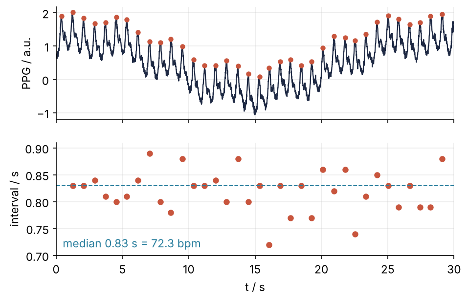
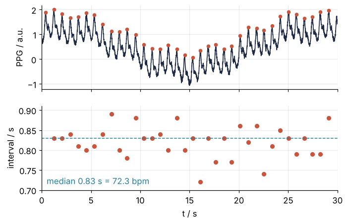
This is where we end up: 36 beats marked on the record, and below it the interval between consecutive beats, whose median of 0.83 s is a rate of 72.3 bpm. The beats were generated at a nominal 72 bpm with some jitter, which came out as a median interval of 0.82 s, or 73.2 bpm. Thirty-seven beats were generated, and the Pitfalls explain the one that is missing. Step 5 explains the difference in rate and draws this figure.

Setup

The cell generates the record. Each beat is a Gaussian bump with its dicrotic wave 0.28 s later, the beats come every 60/72 s with a little jitter, and noise and drift go on top. The drift is two slow waves: a large one with a period of 25 s for the finger pressure, and a smaller one with a period of 4 s for breathing.

import numpy as np
import matplotlib.pyplot as plt
from scipy.signal import find_peaks

plt.rcParams.update({
    "figure.figsize": (7, 3.6), "figure.dpi": 110,
    "axes.spines.top": False, "axes.spines.right": False,
    "axes.grid": True, "grid.alpha": 0.25,
    "font.size": 11, "lines.linewidth": 1.8,
})
INK, ACCENT, SECOND, MUTED = "#1f2a44", "#c8553d", "#2a7f9e", "#8a8f98"

fs = 100                                   # samples per second
t = np.arange(0, 30, 1 / fs)               # s
rng = np.random.default_rng(7)

# The beat times and the drift are known only because we make the signal; with your own
# recording you have t, x, and fs, and nothing else.
t_beats = [0.4]
while True:
    t_next = t_beats[-1] + 60 / 72 + rng.normal(0, 0.03)   # 72 bpm, with jitter
    if t_next >= 30:
        break
    t_beats.append(t_next)
t_beats = np.array(t_beats)

bump = lambda t0, a: a * np.exp(-0.5 * ((t - t0) / 0.09) ** 2)
x = sum(bump(tb, 1.0) + bump(tb + 0.28, 0.4) for tb in t_beats)
drift = 0.8 * np.sin(2 * np.pi * 0.04 * t + 1) + 0.2 * np.sin(2 * np.pi * 0.25 * t)
x += drift
x += rng.normal(0, 0.05, t.size)                                                    # noise, a.u.

ibi_true = np.median(np.diff(t_beats))
print(f"generated {len(t_beats)} beats, the last at {t_beats[-1]:.2f} s; "
      f"median interval {ibi_true:.3f} s = {60 / ibi_true:.1f} bpm")

generated 37 beats, the last at 29.92 s; median interval 0.820 s = 73.2 bpm

Step 1: Call find_peaks and read what comes back

Call it with nothing but the signal, and print what comes back:

peaks, props = find_peaks(x)
print(len(peaks), "peaks")
print("indices:", peaks[:5])
print("times:  ", t[peaks[:5]], "s")
print("props:  ", props)

881 peaks
indices: [ 4  7  9 12 16]
times:   [0.04 0.07 0.09 0.12 0.16] s
props:   {}

find_peaks returns two things: an array of indices into x, and a dictionary of properties. The indices are positions in the array, not times and not values; t[peaks] and x[peaks] turn them into those. Without conditions, a peak is any sample higher than both its neighbors, so the noise alone makes 881 peaks in 3,000 samples, one every three or four samples. The dictionary is empty because no condition was asked for. Steps 3 and 4 fill it.

Step 2: Try a height threshold, and see why it fails here

The obvious fix is a minimum height: keep only the peaks that reach 1.0.

peaks, _ = find_peaks(x, height=1.0)
print(len(peaks), "peaks above 1.0")

268 peaks above 1.0

Every noise wiggle on a crest above the line still counts. Add distance=30, which keeps one peak per crest so that the count can be compared with the 37 beats; Step 5 explains the number. The comparison takes, for each peak, the time since the last generated beat. A beat up to 0.05 s after the peak counts too, because a detected peak can sit slightly before the beat that made it.

Copy

peaks, _ = find_peaks(x, height=1.0, distance=30)
lag = np.array([tp - t_beats[t_beats <= tp + 0.05].max() for tp in t[peaks]])  # s since the last beat
is_beat = lag < 0.05
print(f"{len(peaks)} peaks: {is_beat.sum()} beats, {(~is_beat).sum()} others, "
      f"{lag[~is_beat].min():.2f} to {lag[~is_beat].max():.2f} s after a beat")

fig, ax = plt.subplots()
ax.plot(t, x, color=INK, lw=1.1)
ax.axhline(1.0, color=SECOND, lw=1, ls="--")
ax.text(10.5, 1.08, "height = 1.0", color=SECOND)
ax.plot(t[peaks], x[peaks], "o", color=ACCENT, ms=4)
ax.set(xlabel="t / s", ylabel="PPG / a.u.", xlim=(0, 30))
plt.show()

36 peaks: 23 beats, 13 others, 0.29 to 0.35 s after a beat

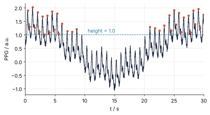
Thirty-six peaks against 37 beats looks nearly right, and it is wrong. Only 23 are beats; the other 13 sit 0.29 to 0.35 s after a beat, which makes them dicrotic waves. That check works only because we made the signal. With your own data the figure is the check: in the middle of the record the drift pulls whole beats under the line, and near both ends it lifts the dicrotic waves over it. A count that looks right proves nothing until you have plotted the peaks on the signal.

height is the right knob on a flat baseline of known scale, such as the amplitude spectrum of the Fourier tutorial, which uses height=0.15, or the filtered ECG in Filtering with scipy.signal: mains hum and noise out of an ECG. It also serves as a floor against noise far below every peak.

Step 3: Measure how far each peak stands out: prominence

What sets a beat apart from a dicrotic wave is not how high it reaches but how far it rises above its surroundings. That quantity takes two moves to define. From the peak, walk along the signal on each side until you meet a higher sample or the end of the record, and note the lowest point of each walk. The higher of these two troughs is the peak's base, and the height of the peak above its base is its prominence.

For a dicrotic wave the walk to the left ends at its own beat, which is higher, so the lowest point on that side is the notch between them. That notch is the higher trough, and the prominence is the small rise out of the notch, however far the drift has lifted the whole wave. A beat is higher than its dicrotic waves and often higher than the beats next to it, so its walks run past all of those and stop only at a beat higher still. The lowest point of each walk is then the foot of some beat it passed, and the base is the higher of those two feet. Ask for prominence=0, which every peak passes, and find_peaks measures it for all of them:

peaks, props = find_peaks(x, prominence=0)
print(list(props))

prom, left, right = props["prominences"], props["left_bases"], props["right_bases"]
base = np.where(x[left] > x[right], left, right)                               # the higher trough
shown = np.flatnonzero((t[peaks] > 11.8) & (t[peaks] < 13.2) & (prom > 0.15))  # skip noise wiggles
for i in shown:
    print(f"peak at {t[peaks[i]]:5.2f} s   prominence {prom[i]:.3f}   "
          f"troughs at {t[left[i]]:5.2f} and {t[right[i]]:5.2f} s   "
          f"drift rise from base {drift[peaks[i]] - drift[base[i]]:+.2f}")

['prominences', 'left_bases', 'right_bases']
peak at 12.03 s   prominence 0.999   troughs at 11.67 and 12.52 s   drift rise from base -0.08
peak at 12.34 s   prominence 0.209   troughs at 12.19 and 12.52 s   drift rise from base +0.03
peak at 12.83 s   prominence 1.306   troughs at 10.96 and 14.97 s   drift rise from base +0.15

Copy

fig, ax = plt.subplots(figsize=(7, 3.2))
ax.plot(t, x, color=INK)
for i in shown:
    p, b = peaks[i], base[i]
    color = ACCENT if prom[i] > 0.5 else MUTED          # a beat is the result; a dicrotic wave is context
    ax.hlines(x[b], t[b], t[p], color=MUTED, lw=1, ls="--")
    ax.vlines(t[p], x[b], x[p], color=color, zorder=3)
    ax.text(t[p], x[p] + 0.04, f"{prom[i]:.2f}", color=color, ha="center", va="bottom")
ax.set(xlabel="t / s", ylabel="PPG / a.u.", xlim=(11.8, 13.2), ylim=(-0.9, 0.8))
plt.show()

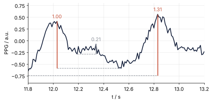
The dicrotic wave at 12.34 s stands 0.209 above the notch at 12.19 s. The beat at 12.83 s takes its base from the left walk, at 10.96 s, two beats back, and its prominence of 1.306 is more than the 1.0 it was generated with: from that trough to the peak the drift rises by 0.15, and the noise at the two ends supplies most of the rest. Prominence ignores how high the drift has carried a peak, but not how much the drift changes between the peak and its base, so every beat comes out a few tenths above or below 1. The dicrotic waves stay far below, and Step 4 turns that gap into a threshold.

Step 4: Choose the threshold from the prominences

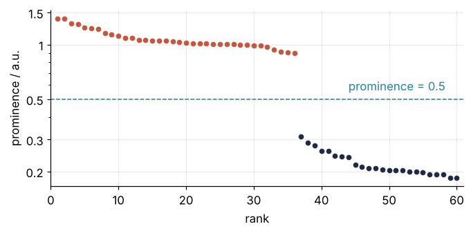
With your own signal you do not know in advance that a beat stands about 1 above its base, so do not guess the threshold. Sort the prominences of all peaks and look for the gap between the peaks you want and the rest:

order = np.argsort(prom)[::-1]                 # largest prominence first
prom_sorted = prom[order]
print(np.round(prom_sorted[:40], 2))
print(f"the 37th, {prom_sorted[36]:.2f}, belongs to the peak at {t[peaks[order[36]]]:.2f} s")

[1.39 1.39 1.31 1.3  1.25 1.23 1.22 1.15 1.13 1.12 1.09 1.09 1.06 1.06
 1.05 1.05 1.05 1.04 1.03 1.03 1.02 1.02 1.01 1.01 1.01 1.01 1.   1.
 1.   0.99 0.99 0.97 0.94 0.91 0.91 0.9  0.31 0.29 0.28 0.26]
the 37th, 0.31, belongs to the peak at 29.93 s

Plotted against rank on a logarithmic axis, so that the small noise prominences stay visible next to the beats, the gap is hard to miss:

Copy

rank = np.arange(1, 61)
above = prom_sorted[:60] > 0.5
fig, ax = plt.subplots(figsize=(7, 3))
ax.semilogy(rank[above], prom_sorted[:60][above], "o", color=ACCENT, ms=4)
ax.semilogy(rank[~above], prom_sorted[:60][~above], "o", color=INK, ms=4)
ax.axhline(0.5, color=SECOND, lw=1, ls="--")
ax.text(44, 0.56, "prominence = 0.5", color=SECOND)
ax.set_yticks([0.2, 0.3, 0.5, 1, 1.5], labels=["0.2", "0.3", "0.5", "1", "1.5"])
ax.yaxis.set_minor_formatter(plt.NullFormatter())    # no 2×10⁻¹ style labels
ax.set(xlabel="rank", ylabel="prominence / a.u.", xlim=(0, 61))
plt.show()

for threshold in [0.35, 0.85]:
    print(f"prominence = {threshold}: {len(find_peaks(x, prominence=threshold)[0])} peaks")

prominence = 0.35: 36 peaks
prominence = 0.85: 36 peaks

Thirty-six prominences run from 1.39 down to 0.90, then the next is 0.31, a factor of three lower, and the rest slide slowly into the noise. Any threshold inside the gap gives the same answer, and the code checks both ends: 0.35 and 0.85 each find 36 peaks. A count that does not move across the gap is the test that a threshold is not a lucky guess. Take a value near the middle, here 0.5, about half a beat. The 37th value belongs to the last beat of the record, and the Pitfalls come back to it. If there is no gap, the peaks you want cannot be told apart by prominence alone, and the next knob to try is width, in Variations.

Step 5: Add a minimum distance and turn peak times into a heart rate

distance is the smallest spacing allowed between two peaks; of two peaks closer than that, find_peaks keeps the taller one. It counts samples, never seconds, so derive it from the fastest rate you believe:

max_rate = 200                             # bpm; no heart in this recording beats faster
distance = round(fs * 60 / max_rate)       # samples
print(f"distance = {distance} samples = {distance / fs:.2f} s")
for threshold in [0.5, 0.2]:
    n_without = len(find_peaks(x, prominence=threshold)[0])
    p = find_peaks(x, prominence=threshold, distance=distance)[0]
    lag = np.array([tp - t_beats[t_beats <= tp + 0.05].max() for tp in t[p]])  # as in Step 2
    print(f"prominence = {threshold}: {n_without} peaks without distance, {len(p)} with, "
          f"{(lag < 0.05).sum()} of them beats")

distance = 30 samples = 0.30 s
prominence = 0.5: 36 peaks without distance, 36 with, 36 of them beats
prominence = 0.2: 53 peaks without distance, 41 with, 37 of them beats

At a good threshold distance changes nothing, 36 peaks either way. At a threshold set too low, 0.2, it brings 53 peaks down to 41: all 37 beats, the one at the edge included, and four dicrotic waves. It is a guard against a split peak or a careless threshold, not a substitute for prominence.

The intervals between beats are the differences of their times, and the rate is 60 s divided by the median interval:

peaks, _ = find_peaks(x, prominence=0.5, distance=distance)
ibi = np.diff(t[peaks])                    # interbeat intervals, s
rate = 60 / np.median(ibi)
print(f"{len(peaks)} beats from {t[peaks[0]]:.2f} to {t[peaks[-1]]:.2f} s")
print(f"median interval {np.median(ibi):.3f} s   rate {rate:.1f} bpm   (generated: {60 / ibi_true:.1f} bpm)")
shift = t[peaks] - t_beats[:len(peaks)]    # the 37th beat, at the edge, is not among them
print(f"detected peak minus generated beat: {1000 * shift.min():+.0f} to {1000 * shift.max():+.0f} ms")

36 beats from 0.42 to 29.11 s
median interval 0.830 s   rate 72.3 bpm   (generated: 73.2 bpm)
detected peak minus generated beat: -23 to +34 ms

Take the median, not the mean: a missed beat makes one double interval, which drags the mean along and leaves the median nearly where it was. The 0.9 bpm between 72.3 and 73.2 bpm is not the sampling, which moves a peak by at most 5 ms. The noise moves the top sample of each crest, and the detected peaks sit from 23 ms before to 34 ms after the beats that made them. Every interval inherits the difference of two such shifts, and here the median lands one sample, 10 ms, above the generated one.

Copy

fig, (ax1, ax2) = plt.subplots(2, 1, sharex=True, figsize=(7, 4.4))
ax1.plot(t, x, color=INK, lw=1.1)
ax1.plot(t[peaks], x[peaks], "o", color=ACCENT, ms=4)
ax1.set(ylabel="PPG / a.u.")
ax2.plot(t[peaks[1:]], ibi, "o", color=ACCENT, ms=5)
ax2.axhline(np.median(ibi), color=SECOND, lw=1, ls="--")
ax2.text(0.5, 0.715, f"median {np.median(ibi):.2f} s = {rate:.1f} bpm", color=SECOND)   # empty corner
ax2.set(xlabel="t / s", ylabel="interval / s", xlim=(0, 30), ylim=(0.70, 0.91))
plt.show()

Pitfalls

A peak at the edge of the record. The symptom is one beat fewer than expected, at the start or the end. Here it is the beat at 29.93 s, 0.07 s before the record stops, missing from the 36. The record ends on its falling slope, so the walk to the right reaches the end before it reaches a trough, and the prominence is only 0.31, the first value below the gap in Step 4. find_peaks also never returns the first or last sample, because a peak needs a neighbor on each side. The rate from intervals does not care: a beat lost at the end costs one interval out of 36. For counts, distrust any peak within a beat's width of either end, and record a little longer than the stretch you want.

distance and width in seconds. find_peaks(x, distance=0.3) raises "distance must be greater or equal to 1", which is the lucky case. The silent case is worse: distance=30, copied from this tutorial to a recording at 250 Hz, means 0.12 s, and the guard is gone without a word. Always write distance=round(fs * min_interval), and the same for width.

Smoothing first, and shifting the peaks. After a moving average "to clean the signal", the peaks sit later than in the raw record. An average over the last k samples, such as pandas' rolling(k).mean() or a hand-written loop over the previous samples, describes the moment (k − 1)/2 samples ago. For k = 15 at 100 Hz that is 7 samples, 70 ms. The rate does not change, but every time you compare with another signal is off. First try prominence on the raw signal; here it already ignores the noise. If you must smooth, use a centered window, np.convolve(x, np.ones(k) / k, mode="same") with odd k, which averages each sample with the (k − 1)/2 samples on either side, or rolling(k, center=True). For real filters, the next step is the filtering tutorial linked in Step 2.

Variations

• Spectral lines. Run find_peaks on an amplitude spectrum with height, and sort the lines by props["peak_heights"], largest first.
• Chromatogram peaks and their widths. Add width= in samples to reject narrow spikes. scipy.signal.peak_widths(x, peaks, rel_height=0.5) gives each peak's width at half its prominence, the first step toward a peak area.
• Troughs instead of peaks. find_peaks(-x, ...) finds the minima, such as the foot of each pulse, the moment the pulse arrives at the finger. The delay from the ECG's R peak to that foot is called the pulse arrival time.
• Peaks in an image. In two dimensions, keep the pixels that equal the maximum of their neighborhood, image == scipy.ndimage.maximum_filter(image, size=w), where w plays the part of distance and a floor on the value that of height. Counting cells with scipy.ndimage: how many are there, and how large? does this on a distance map.

Cheat sheet

peaks, props = find_peaks(x)                       # every local maximum, as indices into x
peaks, props = find_peaks(x, prominence=0)         # measure every prominence, drop nothing
np.sort(props["prominences"])[::-1]                # find the gap, take a threshold in its middle
distance = round(fs * min_interval)                # in samples, never seconds
peaks, _ = find_peaks(x, prominence=p, distance=distance)
find_peaks(x, height=h)                            # only on a flat baseline
find_peaks(x, width=w)                             # w in samples, too
t[peaks], x[peaks]                                 # times and values of the peaks
rate = 60 / np.median(np.diff(t[peaks]))           # per minute, from the median interval

Further reading

• The SciPy reference for scipy.signal.find_peaks and for scipy.signal.peak_prominences, which gives the definition of prominence step by step.
• Steven W. Smith, The Scientist and Engineer's Guide to Digital Signal Processing, free online, for moving averages and their delay.
• John Allen, "Photoplethysmography and its application in clinical physiological measurement", Physiological Measurement 28 (2007) R1, for the PPG waveform and the dicrotic wave.
• Related tutorials on this site: The Fourier transform: asking a signal how much of each frequency it contains and Filtering with scipy.signal: mains hum and noise out of an ECG. Planned: The same heartbeats in Julia with Peaks.jl.
• Download the notebook. It was executed with the library versions in the header.