Genetic drift: why a neutral allele is fixed or lost, and how long it takes (Python)

The question

Take a population of 100 diploid plants on a small island. At one gene they carry 200 copies, and 20 of those copies are a new variant, a new allele of the gene, that neither helps nor harms its carrier: its frequency is p = 0.1. Nothing favors the variant, and yet its frequency does not stay at 0.1. That is genetic drift. Here is one such population followed for 200 generations, each generation made of 200 gene copies drawn at random from the copies of the one before.

Show code

import numpy as np
import matplotlib.pyplot as plt

plt.rcParams.update({
    "figure.figsize": (7, 3.2), "figure.dpi": 110,
    "axes.spines.top": False, "axes.spines.right": False,
    "axes.grid": True, "grid.alpha": 0.25,
    "font.size": 11, "lines.linewidth": 1.8,
})
INK, ACCENT, SECOND, MUTED = "#1f2a44", "#c8553d", "#2a7f9e", "#8a8f98"

TWO_N, K0 = 200, 20                  # gene copies (N = 100 diploid individuals), variant copies at the start
P0 = K0 / TWO_N
SEED = 20261008
rng = np.random.default_rng(SEED)    # one generator for the whole notebook: run the cells in order

k, path = K0, [K0]
for t in range(200):
    k = rng.binomial(TWO_N, k / TWO_N)
    path.append(k)
p_one = np.array(path) / TWO_N
t_peak = p_one.argmax()
t_gone = np.argmax(p_one == 0)
print(f"highest frequency {p_one[t_peak]:.3f} at generation {t_peak}; lost at generation {t_gone}")

fig, ax = plt.subplots()
ax.step(np.arange(p_one.size), p_one, where="post", color=INK)
ax.axhline(P0, color=SECOND, lw=1, ls="--")
ax.text(200, P0 + 0.01, "starting frequency", color=SECOND, ha="right", va="bottom")
ax.annotate(f"lost at generation {t_gone}", (t_gone, 0), xytext=(t_gone + 22, 0.045), va="center",
            arrowprops=dict(arrowstyle="->", color=MUTED, lw=1), color=INK)
ax.set(xlabel="generation", ylabel="variant frequency", xlim=(0, 200), ylim=(-0.01, 0.35))
plt.show()

highest frequency 0.285 at generation 9; lost at generation 52

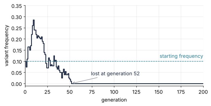
Frequency of a neutral variant in one population of 200 gene copies over 200 generations. It starts at 0.1, wanders up to 0.285 at generation 9, and drops to 0 at generation 52, where it stays.

The frequency jumps by a few percentage points every generation, up as often as down, with no trend. By generation 9 it had climbed to 0.285, almost three times its start, and at generation 52 the last copy was gone. From there on it stays at 0, because a variant that is not in the population cannot be drawn into the next one. Peter Buri saw the same wandering in 1956 in 107 laboratory populations of 16 fruit flies each, bred for 19 generations.

There is no selection here and no mutation after the start, only the sampling of 200 copies from 200. Less obvious: why can the frequency not hover around 0.1 forever, how often does such a variant end up in every copy instead of none, how long does that take, and what happens meanwhile to the genetic variation of the population? Once the variant is lost or fixed, every individual is homozygous at this gene, and the variation is gone.

The idea: every generation is a random sample of the last

Each of the 200 copies of the next generation picks a parent copy at random from the current generation, with replacement, and inherits its type. With k variant copies among 200, each pick is a variant with chance p = k/200, independently of the others. The number of variants in the next generation is then the number of successes in 200 independent tries with success chance p, and that count is what the binomial distribution describes, Binomial(200, p). This is the Wright-Fisher model.

The model ignores which two copies sit together in one individual. Under random mating that pairing does not change the drift. Selfing, an uneven sex ratio, and uneven numbers of offspring do, and they enter through the effective population size below. Hardy-Weinberg's constant allele frequencies hold in an infinite population. Drift is what a finite one adds.

NumPy draws binomial numbers from a seeded generator, as in Random numbers with numpy.random. Here are 100,000 possible next generations of our population:

nxt = rng.binomial(TWO_N, P0, size=100_000)
print(f"variant copies in the next generation: mean {nxt.mean():.1f}, standard deviation {nxt.std():.2f}")
print(f"binomial standard deviation √(2N p (1 − p)) = {np.sqrt(TWO_N * P0 * (1 - P0)):.2f}")

variant copies in the next generation: mean 20.0, standard deviation 4.25
binomial standard deviation √(2N p (1 − p)) = 4.24

On average the next generation has 20.0 variant copies, as many as this one. The standard deviation is 4.25 copies, against √(200 · 0.1 · 0.9) = 4.24 from the formula. One generation moves the count by about four copies, two percentage points of frequency, up or down with equal weight.

The next generation starts from wherever this one landed, and the following draw adds its own step. The steps pile up like those of the random walk in the prerequisite, with one difference: this walk has two walls it cannot leave. Once k reaches 0, every pick is the old type and no draw brings the variant back. Once k reaches 200, no draw removes it. A frequency that keeps wandering must sooner or later hit one of the walls, and there it stays.

Follow 20,000 populations, all started at 0.1, and look at the distribution of their frequencies at three moments:

Show code

R = 20_000
k = np.full(R, K0)
snapshots, means = {}, {}
for t in range(1, 1001):
    k = rng.binomial(TWO_N, k / TWO_N)
    if t in (1, 10, 50, 200, 1000):
        snapshots[t] = k.copy()
        means[t] = (k / TWO_N).mean(), (k / TWO_N).std() / np.sqrt(R)

# bins of five copy numbers, with edges between attainable counts so that no bin gets an extra one
bins = np.append(np.arange(0.5, TWO_N, 5), TWO_N - 0.5) / TWO_N
fig, axes = plt.subplots(3, 1, figsize=(7, 6), sharex=True)
for ax, t in zip(axes, (10, 50, 200)):
    f = snapshots[t] / TWO_N
    inside = f[(f > 0) & (f < 1)]
    counts, _ = np.histogram(inside, bins=bins)
    share = counts / R * np.append(np.ones(counts.size - 1), 5 / 4)   # the last bin holds four counts, 196 to 199
    ax.stairs(share, bins, fill=True, color=ACCENT, alpha=0.8, lw=0)
    ax.axvline(P0, color=SECOND, lw=1, ls="--")
    ax.set_ylim(0, 1.5 * share.max())                      # headroom for the labels
    ax.text(0.99, 0.95, f"generation {t}:  lost {100 * np.mean(f == 0):.1f} %,  fixed {100 * np.mean(f == 1):.1f} %",
            transform=ax.transAxes, va="top", ha="right", color=INK)
    ax.set_ylabel("share of\npopulations")
axes[0].text(P0 + 0.01, 0.95, "start", transform=axes[0].get_xaxis_transform(), color=SECOND, va="top")
axes[-1].set(xlabel="variant frequency", xlim=(0, 1))
plt.show()

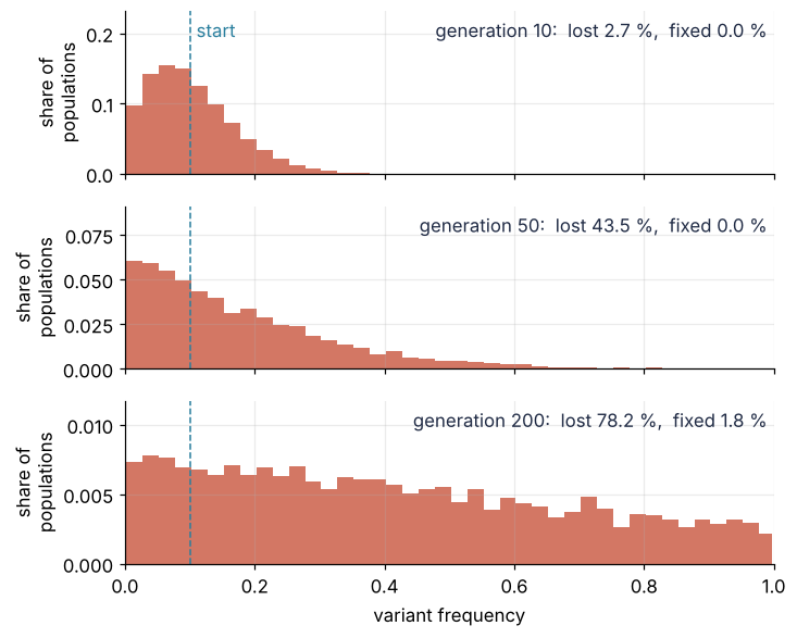
Share of 20,000 populations, all started at frequency 0.1, against variant frequency, after 10, 50, and 200 generations. The hump spreads and flattens while the populations drain into the edges: 2.7, 43.5, and 78.2 % lost, and 1.8 % fixed by generation 200.

After 10 generations the populations form a hump around 0.1, and 2.7 % of them have already lost the variant. After 50 the hump reaches over half the range and 43.5 % have lost it. After 200 it is flat and low, 78.2 % have lost the variant, and the first populations, 1.8 %, carry it in every copy. A population that leaves the hump goes to one of the edges and never comes back.

The animation runs the same experiment for 1,500 generations. Above, 50 populations step from generation to generation, and a line turns from gray to red the moment its variant is fixed. Below, the distribution of 20,000 populations spreads out and drains, mostly to the left edge and a little to the right, until at generation 1,500 only 6 of the 20,000 are left in between. Keep an eye on the blue line, the mean frequency, while everything around it moves.

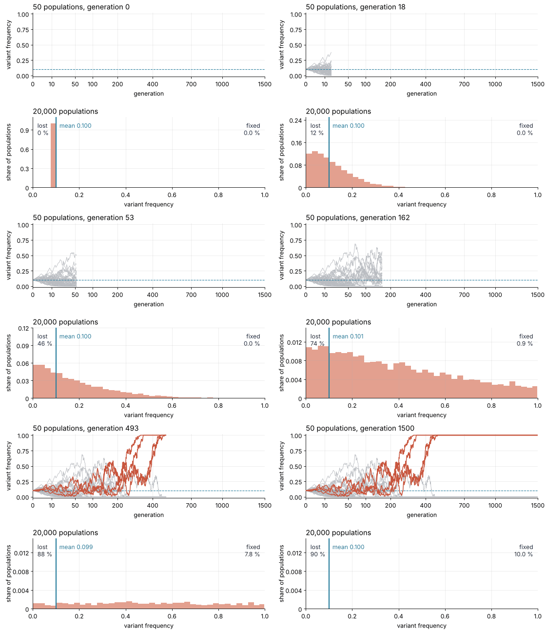
Animation over 1,500 generations. Top: 50 allele-frequency trajectories wander from 0.1; most drop to 0, a few reach 1 and turn red. Bottom: the frequency distribution of 20,000 populations spreads and drains into lost and fixed, while its mean, a blue line, stays at 0.1.

How I built this: each frame advances every population by one or more binomial generations and redraws the trajectories and the histogram with Matplotlib's FuncAnimation, the technique of Matplotlib animation with FuncAnimation; the source is animations/frequency-spread/scene.py.

Why the chance to win is the starting frequency

The hump spreads, but its center does not move. Here is the mean frequency of the same 20,000 populations at five generations:

Show code

for t, (m, se) in means.items():
    print(f"generation {t:5d}: mean frequency {m:.4f} ± {se:.4f}")

generation     1: mean frequency 0.1002 ± 0.0001
generation    10: mean frequency 0.1006 ± 0.0005
generation    50: mean frequency 0.0987 ± 0.0010
generation   200: mean frequency 0.1003 ± 0.0017
generation  1000: mean frequency 0.0967 ± 0.0021

It stays at 0.1 within the scatter of an average of 20,000 numbers, the standard error printed beside it (The standard error of the mean explains the ±). A simulated average lands within two standard errors of its true value in 95 % of runs, so the 0.0967 at generation 1,000, 1.6 standard errors low, is scatter, not a trend. The reason is in the binomial draw: its expected value is 200p copies, so the expected frequency of the next generation is exactly the current one. Drift has no direction.

Run long enough and every population ends at 0 or 1. The mean frequency is then the share of populations at 1, the fraction fixed. Since the mean never moved, that fraction is 0.1: a neutral variant wins with exactly its starting frequency. A quantity whose expected next value is its current value is called a martingale, the mathematical word for a fair game. A fair game cannot be won on average, only ended.

The time it takes follows from the size of the steps. One generation adds p(1 − p)/2N = 0.00045 to the variance of the frequency: the standard deviation of 4.25 copies from the 100,000 draws, divided by 200 copies, is 0.0213 in frequency, and 0.0213² is 0.00045. Independent steps add their variances, which is why the mean squared distance of the prerequisite's random walk grows in proportion to the number of steps. A set of populations split between 0 and 1, a share p of them at 1, has the variance p(1 − p), and at p(1 − p)/2N per generation the spread needs a number of generations proportional to 2N to get there. The factor in front comes in the Formalization. Double the population and the wait doubles.

Formalization

The model is a chain of binomial draws. With k variant copies among 2N, the chance that the next generation has j of them is

\[P(k \to j) = \binom{2N}{j} \left(\frac{k}{2N}\right)^{j} \left(1 - \frac{k}{2N}\right)^{2N - j},\]

the Wright-Fisher transition probability, where N is the number of diploid individuals and $\binom{2N}{j}$ counts the ways to choose which j of the 2N picks are variants. Two moments of it, its mean and its variance, carry everything that follows. For the frequency p' = j/2N of the next generation,

\[E[p'] = p, \qquad \operatorname{Var}(p') = \frac{p(1-p)}{2N}.\]

In the example the first is 0.1 and the second 0.00045, a standard deviation of 0.021. The states p = 0 and p = 1 are the absorbing states of the chain: once there, the chain stays with probability 1.

Three consequences follow that you need every time.

The fixation probability is the starting frequency. For a neutral allele in this model, u(p) = p exactly, by the fair-game argument of the section before, so u = 0.1 here. A new mutation starts as one copy among 2N and wins with probability 1/2N, 0.005 in our population. Of every 200 new neutral mutations, 199 are lost on average.

A winner takes about 4N generations. Kimura and Ohta (1969) gave the mean time to fixation for the alleles that do fix,

\[\bar t(p) = -\frac{4N(1-p)\ln(1-p)}{p},\]

379 generations for N = 100 and p = 0.1, and 399, close to 4N = 400, for a single new copy, p = 1/2N. The formula is a diffusion approximation: it treats the frequency as a continuous quantity, which is accurate when 2N is large. That the time is proportional to N you already know from the step sizes; the formula supplies the factor in front.

Mean heterozygosity decays by 1/2N per generation. The heterozygosity of a population, H = 2p(1 − p), is the chance that two copies drawn from it at random, with replacement, differ. It is also the Hardy-Weinberg share of heterozygous individuals, here H₀ = 2 · 0.1 · 0.9 = 0.18. One population's H jumps around with its p and ends at 0. Its average over many populations, the mean heterozygosity H̄ₜ, falls smoothly:

\[\bar H_t = H_0 \left(1 - \frac{1}{2N}\right)^t .\]

The reason is in the two copies. Pick two from the next generation, with replacement. With chance 1/2N it is the same copy twice, and a copy cannot differ from itself. Otherwise they are two different copies whose parents were drawn independently from the current generation, so they differ with exactly the chance Hₜ. On average, then, H̄ₜ₊₁ = (1 − 1/2N) H̄ₜ, and t generations multiply the factors. At t = 100 the mean heterozygosity is 0.109. For a small x, 1 − x is close to $e^{-x}$, so the factor after t generations is about $e^{-t/2N}$, and the mean heterozygosity halves every 2N ln 2 ≈ 138 generations.

Every N above is the effective population size Nₑ, the size of the ideal Wright-Fisher population that drifts as fast as the real one. Real populations usually have an Nₑ below their census size, and changing numbers are the easiest reason to compute.

Each generation keeps the fraction 1 − 1/2Nₜ of the heterozygosity. With the same approximation, T generations keep about $\exp(-\sum_t 1/2N_t)$, so what adds up is 1/Nₜ. A constant population of size Nₑ loses as much only if T/Nₑ equals the sum of the 1/Nₜ, which makes Nₑ the number of generations divided by the sum of the inverse sizes: the harmonic mean. A population of 1,000 that crashes to 10 for one generation in five has Nₑ = 5/(4/1000 + 1/10) ≈ 48, not the arithmetic mean of 802: the one generation at 10 contributes 25 times more to the sum than the four at 1,000 together.

The predictions for the example, which the next section tests:

Show code

N = TWO_N // 2
u_theory = P0
t_fix_theory = lambda n, p: -4 * n * (1 - p) * np.log(1 - p) / p
H0 = 2 * P0 * (1 - P0)
print(f"fixation probability       u = {u_theory:.3f}")
print(f"mean fixation time         t = {t_fix_theory(N, P0):.1f} generations")
print(f"mean heterozygosity at 100 H = {H0 * (1 - 1 / TWO_N) ** 100:.4f}")
print(f"half-life of heterozygosity    {np.log(2) / -np.log(1 - 1 / TWO_N):.1f} generations")
print(f"Nₑ of 1000, 1000, 1000, 1000, 10: {5 / (4 / 1000 + 1 / 10):.1f}")

fixation probability       u = 0.100
mean fixation time         t = 379.3 generations
mean heterozygosity at 100 H = 0.1090
half-life of heterozygosity    138.3 generations
Nₑ of 1000, 1000, 1000, 1000, 10: 48.1

See it in code

rng.binomial accepts an array of probabilities, so one call advances all 20,000 populations by a generation. The cell below runs them until every one is decided, records when each was fixed or lost, and repeats the run at 2N = 100 and 400.

Show code

def drift(two_n, R, keep=0, t_max=1000):
    """Wright-Fisher populations started at frequency 0.1, run until every one is fixed or lost."""
    k = np.full(R, two_n // 10)
    t_decided = np.zeros(R, dtype=int)
    frac_fixed, H_mean, paths = [0.0], [np.mean(2 * k / two_n * (1 - k / two_n))], [k[:keep] / two_n]
    H_se = [0.0]
    t = 0
    while np.any((k > 0) & (k < two_n)):
        t += 1
        open_ = (k > 0) & (k < two_n)
        k = rng.binomial(two_n, k / two_n)
        t_decided[open_ & ((k == 0) | (k == two_n))] = t
        if t <= t_max:
            f = k / two_n
            H = 2 * f * (1 - f)
            frac_fixed.append(np.mean(k == two_n))
            H_mean.append(H.mean())
            H_se.append(H.std() / np.sqrt(R))
            paths.append(f[:keep])
    return dict(fixed=k == two_n, t=t_decided, last=t, frac_fixed=np.array(frac_fixed),
                H_mean=np.array(H_mean), H_se=np.array(H_se), paths=np.array(paths))

run = drift(TWO_N, R, keep=50)
fixed, t_dec = run["fixed"], run["t"]
u = fixed.mean()
t_fix, t_loss = t_dec[fixed], t_dec[~fixed]
print(f"fraction fixed        {u:.4f} ± {np.sqrt(u * (1 - u) / R):.4f}   theory {u_theory:.4f}")
print(f"mean fixation time    {t_fix.mean():.1f} ± {t_fix.std(ddof=1) / np.sqrt(t_fix.size):.1f}"
      f"   theory {t_fix_theory(N, P0):.1f}   median {np.median(t_fix):.0f}")
print(f"mean loss time        {t_loss.mean():.1f} ± {t_loss.std(ddof=1) / np.sqrt(t_loss.size):.1f}")
print(f"last population decided at generation {run['last']:,}")
print(f"mean heterozygosity at 100: {run['H_mean'][100]:.4f} ± {run['H_se'][100]:.4f}"
      f"   theory {H0 * (1 - 1 / TWO_N) ** 100:.4f}")

# ---- the figure: 50 trajectories, the fraction fixed, the heterozygosity
gen = np.arange(run["paths"].shape[0])
shown_fixed, shown_t = fixed[:50], t_dec[:50]
print(f"fixed among the 50 drawn: {shown_fixed.sum()}")
fig, (ax1, ax2, ax3) = plt.subplots(3, 1, figsize=(7, 6.4), sharex=True)
for j in range(50):
    ax1.plot(gen, run["paths"][:, j], color=ACCENT if shown_fixed[j] else MUTED,
             lw=1.2 if shown_fixed[j] else 0.8, alpha=1 if shown_fixed[j] else 0.5,
             zorder=3 if shown_fixed[j] else 2)
ax1.text(990, 0.88, f"{shown_fixed.sum()} fixed", color=ACCENT, ha="right", va="top")
ax1.text(990, 0.06, f"{50 - shown_fixed.sum()} lost", color=MUTED, ha="right", va="bottom")
ax1.set(ylabel="variant\nfrequency", ylim=(-0.02, 1.02))

ax2.plot(gen, run["frac_fixed"], color=ACCENT)
ax2.axhline(P0, color=SECOND, lw=1, ls="--")
ax2.text(10, P0 + 0.004, "starting frequency", color=SECOND, va="bottom")
ax2.axvline(t_fix.mean(), color=MUTED, lw=1, ls="--")
ax2.text(t_fix.mean() + 10, 0.02, f"mean fixation time {t_fix.mean():.0f}", color=MUTED)
ax2.set(ylabel="fraction\nfixed", ylim=(0, 0.125))

# three single populations among the 50: the first to fix, and the two lost last within the plotted range
first_fixed = np.flatnonzero(shown_fixed)[np.argmin(shown_t[shown_fixed])]
late_lost = [j for j in np.argsort(-shown_t) if not shown_fixed[j] and shown_t[j] <= gen[-1]][:2]
for j in [first_fixed, *late_lost]:
    f = run["paths"][:, j]
    ax3.plot(gen, 2 * f * (1 - f), color=MUTED, lw=0.9)
ax3.plot(gen, H0 * (1 - 1 / TWO_N) ** gen, color=INK, zorder=3)
ax3.plot(gen[::40], run["H_mean"][::40], "o", ms=4, color=ACCENT, zorder=4)   # every 40th generation
white = dict(fc="white", ec="none", pad=1)                 # labels stay readable over the single populations
ax3.text(450, 0.125, "mean of 20,000 populations (dots)", color=ACCENT, va="bottom", bbox=white)
ax3.text(450, 0.04, r"theory $0.18\,(1 - 1/200)^t$", color=INK, va="bottom", bbox=white)
ax3.text(990, 0.55, "single populations", color=MUTED, ha="right")
ax3.set(ylabel="heterozygosity\nH", xlabel="generation", xlim=(0, 1000), ylim=(0, 0.64))
plt.show()

# ---- the clock: the same run at half and twice the population
print("\n  2N   fraction fixed   mean fixation time   Kimura-Ohta")
for two_n in (100, 200, 400):
    r = run if two_n == TWO_N else drift(two_n, R)
    tf = r["t"][r["fixed"]]
    uf = r["fixed"].mean()
    print(f"{two_n:4d}   {uf:.3f} ± {np.sqrt(uf * (1 - uf) / R):.3f}    "
          f"{tf.mean():6.1f} ± {tf.std(ddof=1) / np.sqrt(tf.size):4.1f}        {t_fix_theory(two_n / 2, 0.1):6.1f}")

fraction fixed        0.0999 ± 0.0021   theory 0.1000
mean fixation time    378.9 ± 4.7   theory 379.3   median 331
mean loss time        99.2 ± 1.0
last population decided at generation 2,209
mean heterozygosity at 100: 0.1075 ± 0.0012   theory 0.1090
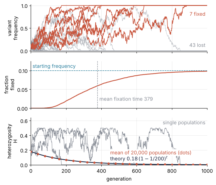
fixed among the 50 drawn: 7

$Three panels against generation, 0 to 1,000. Top: 50 simulated allele-frequency trajectories, 7 fixed in red and 43 lost in gray. Middle: the fraction of 20,000 populations fixed, rising to 0.098 by generation 1,000, just under the starting frequency 0.1. Bottom: the mean heterozygosity on the curve 0.18(1 − 1/200)^t, while three single populations jump and fall to 0.$

  2N   fraction fixed   mean fixation time   Kimura-Ohta
 100   0.100 ± 0.002     185.4 ±  2.4         189.6
 200   0.100 ± 0.002     378.9 ±  4.7         379.3
 400   0.101 ± 0.002     743.2 ±  9.5         758.6

The fraction fixed is 0.0999 ± 0.0021 against the predicted 0.1, and the mean fixation time 378.9 ± 4.7 generations against 379. The lost variants went about four times faster, in 99.2 generations on average. The mean hides a long tail: the median fixation time is 331 generations, and the last population was decided only at generation 2,209. Of the 50 trajectories drawn, 7 fixed where 5 were expected, well within the scatter of 50 tries. In the bottom panel the mean heterozygosity lies on the theory curve, 0.1075 ± 0.0012 against 0.1090 at generation 100, while single populations jump about and drop to 0.

The table is the clock. Each doubling of the population doubles the mean fixation time, 185, 379, 743 generations against the predicted 190, 379, 759, each within two standard errors, while the fraction fixed stays at 0.1.

Where it shows up

Conservation genetics. The northern elephant seal was hunted down to about 20 to 30 animals in the 1890s and numbers about 225,000 today, yet allozyme surveys find a single variant at every gene they examined. At N = 25 one generation removes 2 % of the heterozygosity, at 225,000 about 0.0002 %, so the bottleneck generations dominate the harmonic mean, and what was lost then does not come back with the numbers.
Human and medical genetics. A small founding group carries some alleles at frequencies far from those of the population it left, the founder effect. Among the Old Order Amish of Lancaster County, Ellis-van Creveld syndrome traces back to one couple who arrived in the 18th century, and drift in a small community that marries within itself carried the allele from that couple's copies to the frequency it has there now.
Molecular evolution. With μ the neutral mutation rate per gene copy per generation, 2Nμ new neutral mutations arise each generation and each fixes with probability 1/2N. The rate of substitution is therefore μ, whatever the population size, which is the neutral molecular clock of Kimura (1968).
Phylogenetics. A gene tree is the family tree of the copies of one gene, traced back through the species. When speciations follow each other faster than drift fixes alleles, gene trees disagree with the species tree, incomplete lineage sorting, and for humans, chimpanzees, and gorillas this holds for about 30 % of the genome.
Microbiology and experimental evolution. A serial transfer culture passes a small sample of its cells to fresh medium every day, 1 in 100 in Lenski's long-term E. coli experiment, running since 1988. That daily bottleneck sets the Nₑ of the culture and decides which neutral mutations drift to fixation.

In every case the N that sets the pace of drift is Nₑ, and the smallest numbers a population passed through decide it, not its head count today.

The question

The idea: every generation is a random sample of the last

Why the chance to win is the starting frequency

Formalization

See it in code

Where it shows up

Further reading