The standard error of the mean: why four times the data halves the error

The question

A synthesis is run in twelve batches, and every batch is weighed. The twelve yields have a mean of 49.43 mg, a standard deviation of 2.28 mg, and a standard error of the mean of 0.66 mg, the two numbers people reach for when they draw error bars. Then the lab runs 36 more batches. Here are the twelve, and all 48:

Show code

Copy

import numpy as np
import matplotlib.pyplot as plt
from scipy import stats

plt.rcParams.update({
    "figure.figsize": (7, 3.2), "figure.dpi": 110,
    "axes.spines.top": False, "axes.spines.right": False,
    "axes.grid": True, "grid.alpha": 0.25,
    "font.size": 11, "lines.linewidth": 1.8,
})
INK, ACCENT, SECOND, MUTED = "#1f2a44", "#c8553d", "#2a7f9e", "#8a8f98"

# The batches are simulated from a known truth and rounded like a balance reading.
MU, SIGMA = 50.0, 2.5                                   # mg
twelve = np.round(np.random.default_rng(159).normal(MU, SIGMA, 12), 1)
more = np.round(np.random.default_rng(41).normal(MU, SIGMA, 36), 1)
batches48 = np.concatenate([twelve, more])

for x in [twelve, batches48]:
    print(f"{x.size:2d} batches: mean {x.mean():6.2f} mg   sd {x.std(ddof=1):4.2f} mg   "
          f"standard error {stats.sem(x):4.2f} mg")

fig, ax = plt.subplots()
offsets = np.tile([0.30, 0.42, 0.54, 0.36, 0.48, 0.60], 8)   # fixed heights, so dots do not hide each other
for row, x in zip([1, 0], [twelve, batches48]):
    m, sd, se = x.mean(), x.std(ddof=1), stats.sem(x)
    ax.plot(x, row + offsets[:x.size], "o", color=INK, ms=4)
    ax.plot([m - sd, m + sd], [row + 0.12] * 2, color=SECOND, lw=1.4, solid_capstyle="butt")
    ax.plot([m - se, m + se], [row + 0.02] * 2, color=ACCENT, lw=4, solid_capstyle="butt")
    ax.text(m + sd + 0.2, row + 0.12, f"sd {sd:.2f} mg", color=SECOND, va="center")
    ax.text(m + sd + 0.2, row + 0.00, f"standard error {se:.2f} mg", color=ACCENT, va="center")
ax.set(xlabel="yield / mg", yticks=[0.35, 1.35], yticklabels=["48 batches", "12 batches"],
       xlim=(43.5, 58.5), ylim=(-0.15, 1.8))
ax.grid(axis="y", visible=False)
plt.show()

12 batches: mean  49.43 mg   sd 2.28 mg   standard error 0.66 mg
48 batches: mean  50.02 mg   sd 2.30 mg   standard error 0.33 mg

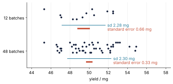
Two things are obvious. The dots of both rows cover the same range, and the standard deviation hardly moves, from 2.28 to 2.30 mg. More batches do not make the batches less scattered, and nobody expects them to.

Less obvious: the standard error moved, from 0.66 to 0.33 mg. Four times the data, and the error fell to half, not to a quarter. The two numbers measure different things: the standard deviation describes the batches, and the standard error describes their mean. So what does the standard error measure, and why does four times the data halve it?

Two facts first, because the rest of the page leans on them. The batches are simulated from a known truth, a mean μ = 50.0 mg and a standard deviation σ = 2.5 mg, rounded to 0.1 mg like a balance reading, so the 2.28 mg is an estimate of σ from twelve values, which I call s. A sample standard deviation divides by n − 1, not by n, and NumPy does that only when asked, with ddof=1. Read the batches as any repeated measurement you average, titrations or grain ages.

The twelve are the standard-protocol batches of scipy.stats from the ground up, drawn with its seed; its Step 1 has the whole ddof trap. For the other 36 I picked seed 41, because it shows the halving cleanly. With any one data set the standard error halves only roughly, and the simulations below draw fresh numbers, so nothing on this page rests on that pick.

The idea: repeat the experiment and look at the means

One experiment of twelve batches gives one mean, 49.43 mg. Run the whole experiment again, twelve fresh batches, and the mean comes out somewhere else. Repeat it many times and the means scatter around 50 mg as well, only less than the batches do. The standard error of the mean is the standard deviation of those means, over many repetitions of the whole experiment. One experiment cannot repeat itself, so it estimates that number from its own scatter, as s/√n.

Why the means scatter less: averaging lets high and low batches cancel. A single batch misses 50 mg by more than 1 mg quite often. For the mean of twelve to miss by that much, most of the twelve have to be off in the same direction, and that gets rare quickly as n grows. Since the truth is known, the computer can run the experiment ten thousand times and count:

sim = np.random.default_rng(2026)

def experiments(n, R=10_000):
    """R repeated experiments of n batches each, drawn from the truth: an (R, n) array in mg."""
    return sim.normal(MU, SIGMA, (R, n))

for n in [1, 12, 48]:
    means = experiments(n).mean(axis=1)
    off = np.mean(np.abs(means - MU) > 1.0)
    print(f"n = {n:2d}: {100 * off:4.1f} % of {means.size:,} means miss 50 mg by more than 1 mg")

n =  1: 70.0 % of 10,000 means miss 50 mg by more than 1 mg
n = 12: 17.0 % of 10,000 means miss 50 mg by more than 1 mg
n = 48:  0.5 % of 10,000 means miss 50 mg by more than 1 mg

Seven single batches in ten miss by more than 1 mg, about one 12-batch mean in six, and one 48-batch mean in two hundred. Cancellation does a lot of work.

Do not expect the 0.66 mg of the opening in the pictures that follow. Both numbers are a standard deviation divided by √12, and the next section derives the √12. The simulation draws from the truth, so its 12-batch means scatter by 2.5/√12 = 0.72 mg. The twelve real batches know only their own s and estimate the same quantity as 2.28/√12 = 0.66 mg. Neither is wrong: 0.72 mg is the truth, and 0.66 mg is what one experiment can say about it.

Here are 10,000 means at three sizes of experiment, each histogram over the curve of single batches:

Show code

Copy

x_grid = np.linspace(43, 57, 400)
batch_curve = np.exp(-0.5 * ((x_grid - MU) / SIGMA) ** 2) / (SIGMA * np.sqrt(2 * np.pi))
bins = np.arange(43, 57.01, 0.2)

fig, axes = plt.subplots(3, 1, figsize=(7, 6.3), sharex=True, sharey=True)   # one y scale: the curve stays put
for ax, n in zip(axes, [3, 12, 48]):
    means = experiments(n).mean(axis=1)
    ax.hist(means, bins=bins, density=True, color=ACCENT, alpha=0.6, lw=0)   # area 1, like the curve
    ax.plot(x_grid, batch_curve, color=INK)
    ax.axvline(MU, color=MUTED, lw=1, ls="--")
    ax.text(0.99, 0.92, f"n = {n}, sd of means {means.std():.2f} mg",
            transform=ax.transAxes, ha="right", va="top", color=ACCENT)
    ax.set(yticks=[])
axes[1].set(ylabel="share per mg")
axes[0].text(43.1, 0.07, "single batches", color=INK, va="bottom")   # above the curve's left tail
axes[-1].set(xlabel="yield / mg", xlim=(43, 57))
plt.show()

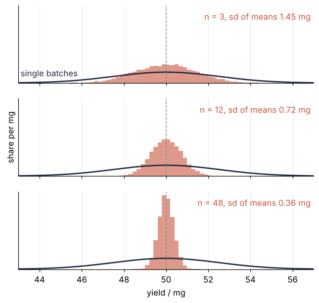
The histograms and the batch curve are both scaled so that their area is 1, which lets them share an axis, and all three panels use the same scale, so a histogram half as wide stands twice as tall. The dashed line is the true mean, 50 mg. Going from 12 to 48 batches halves the width of the histogram, from 0.72 to 0.36 mg. Going from 3 to 12 halves it as well, from 1.45 to 0.72 mg. The curve of single batches underneath never changes.

Watch one histogram build up, experiment by experiment:

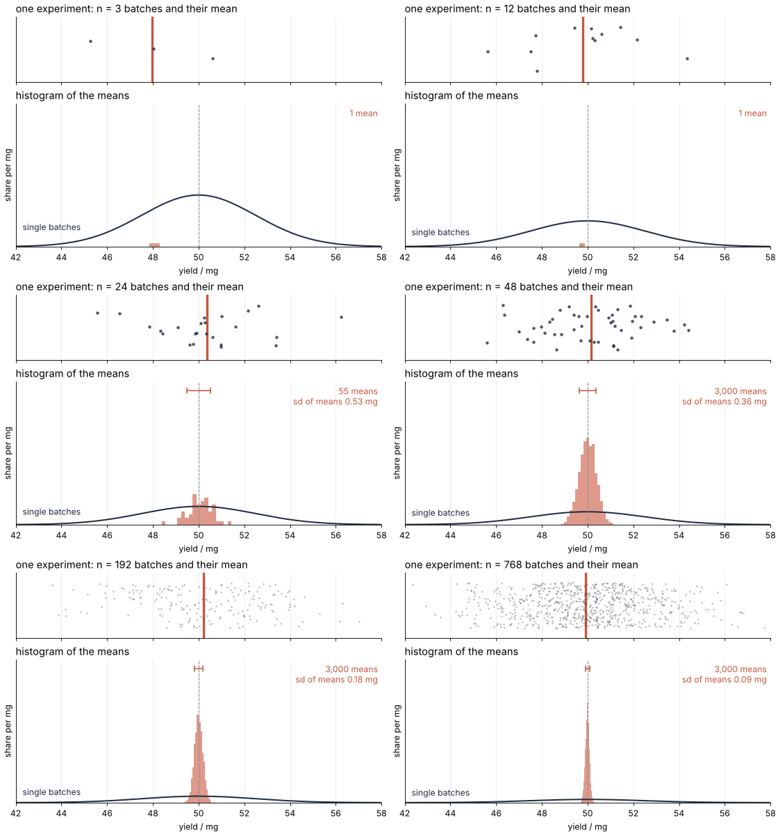
How I built this: each frame draws more experiments and adds their means to the histogram with Matplotlib's FuncAnimation, the technique of Matplotlib animation with FuncAnimation; the source is animations/means-narrowing/scene.py.

The top panel is one experiment, its batches as dots and its mean as a bar. The first means land anywhere near 50 mg, and only after a few hundred experiments does the histogram take its shape. Then n doubles, the histogram starts again, and it fills up narrower than before, with the batches in the top panel exactly as scattered as they were.

Every factor of four in n halves the standard deviation of the means. That is a 1/√n law, not 1/n, and it is what the next section explains.

Formalization

The variance of a set of values is the square of its standard deviation: the average squared distance from the mean, in squared units, so σ = 2.5 mg is a variance of 6.25 mg². The derivation works with variances because they obey two rules that standard deviations do not.

Rule 1: variances of independent values add. When knowing one value tells you nothing about the other, \(\operatorname{Var}(X_1 + X_2) = \operatorname{Var}(X_1) + \operatorname{Var}(X_2)\).

Rule 2: scaling a value by c scales its variance by c². The variance is in squared units, so halving every value quarters it: \(\operatorname{Var}(cX) = c^2 \operatorname{Var}(X)\).

Both rules can be checked on 100,000 simulated pairs of batches:

pair = sim.normal(MU, SIGMA, (100_000, 2)).sum(axis=1)       # two independent batches, added
print(f"Var(X1 + X2)       = {pair.var():6.3f} mg²   rule 1: 2 × 6.25 = 12.500 mg²")
print(f"Var((X1 + X2) / 2) = {(pair / 2).var():6.3f} mg²   rule 2: 12.5 / 4 =  3.125 mg²")

Var(X1 + X2)       = 12.596 mg²   rule 1: 2 × 6.25 = 12.500 mg²
Var((X1 + X2) / 2) =  3.149 mg²   rule 2: 12.5 / 4 =  3.125 mg²

The simulated sum has a variance of 12.6 mg² against 12.5 for rule 1, and half the sum 3.15 mg² against 3.125 for rule 2, both within the scatter of 100,000 draws.

Now the mean of n batches, \(\bar x = (X_1 + \dots + X_n)/n\). By rule 1 the sum of n independent batches has n times the variance of one. Dividing by n is scaling by c = 1/n, which by rule 2 divides the variance by n². The square root brings it back to a standard deviation:

Here σ is the standard deviation of one batch and SE the standard error of the mean. For twelve batches it is the 0.72 mg of the middle histogram.

Why √n and not n: the sum of n batches has n times the variance, but only √n times the standard deviation. The random errors partly cancel, and their sum wanders away from zero like a random walk, about √n step lengths from the start after n steps, the law behind the walkers of Random numbers with numpy.random. Dividing that sum by n leaves √n/n = 1/√n.

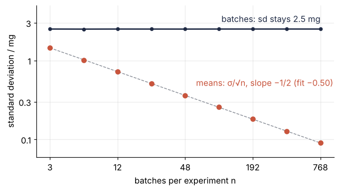
The simulation, swept from 3 to 768 batches per experiment:

ns = 3 * 2 ** np.arange(9)                                   # 3, 6, 12, ..., 768
sd_means, sd_batches = [], []
print("   n   sd of the means   σ/√n       sd of the batches")
for n in ns:
    X = experiments(n)
    # ddof does not matter here: with 10,000 values or more, n and n - 1 differ by under 0.01 %
    sd_means.append(X.mean(axis=1).std())
    sd_batches.append(X.std())
    print(f"{n:4d}   {sd_means[-1]:6.3f} mg       {SIGMA / np.sqrt(n):6.3f} mg   {sd_batches[-1]:6.3f} mg")
sd_means, sd_batches = np.array(sd_means), np.array(sd_batches)

slope, _ = np.polyfit(np.log(ns), np.log(sd_means), 1)
worst = np.max(np.abs(sd_means / (SIGMA / np.sqrt(ns)) - 1))
print(f"fitted slope on log-log axes: {slope:.2f}   largest miss against σ/√n: {100 * worst:.1f} %")

   n   sd of the means   σ/√n       sd of the batches
   3    1.452 mg        1.443 mg    2.501 mg
   6    1.013 mg        1.021 mg    2.495 mg
  12    0.724 mg        0.722 mg    2.500 mg
  24    0.507 mg        0.510 mg    2.498 mg
  48    0.358 mg        0.361 mg    2.497 mg
  96    0.256 mg        0.255 mg    2.501 mg
 192    0.182 mg        0.180 mg    2.501 mg
 384    0.127 mg        0.128 mg    2.502 mg
 768    0.091 mg        0.090 mg    2.500 mg
fitted slope on log-log axes: -0.50   largest miss against σ/√n: 0.8 %

Every row of the table agrees with σ/√n to within 1 %, and the fitted slope on log-log axes is −0.50. A power law \(n^k\) is a straight line of slope k on such axes, so the means fall as \(n^{-1/2} = 1/\sqrt{n}\). The batch column stays at 2.50 mg from 3 batches to 768: a larger experiment measures the mean better, and it does not make the batches better.

Show code

Copy

fig, ax = plt.subplots(figsize=(7, 3.6))
ax.loglog(ns, sd_batches, "o-", color=INK, ms=4)
ax.loglog(ns, SIGMA / np.sqrt(ns), color=MUTED, lw=1, ls="--")
ax.loglog(ns, sd_means, "o", color=ACCENT, ms=6)
ax.text(ns[-1], 2.9, "batches: sd stays 2.5 mg", color=INK, ha="right", va="bottom")
ax.text(60, 0.45, f"means: σ/√n, slope −1/2 (fit {slope:.2f})".replace("-", "−"), color=ACCENT, va="bottom")
ax.minorticks_off()
ax.set(xlabel="batches per experiment n", ylabel="standard deviation / mg", ylim=(0.06, 5),
       xticks=ns[::2], xticklabels=[str(n) for n in ns[::2]],
       yticks=[0.1, 0.3, 1, 3], yticklabels=["0.1", "0.3", "1", "3"])
plt.show()

Three consequences follow, and you will meet each of them every time you average.

A tenth of the error costs a hundred times the data. To bring the standard error from 0.72 mg at twelve batches down to 0.072 mg takes 1,200 batches, because √100 = 10.

In practice σ is estimated. One experiment does not know σ, so the standard error it reports is s/√n, the estimate behind the opening's 0.66 mg. What it is for is an interval. Repeat the experiment many times, and the interval mean ± 2σ/√n contains the true μ in about 95 % of the repetitions. That is a statement about experiments, not about batches: 95 % of single batches lie within ±2σ, an interval √12 = 3.5 times as wide for twelve batches. With s in place of σ the factor 2 grows to 2.20 for twelve batches, because s is itself uncertain; the next section computes it and checks it.

Only independent errors average away. Give every batch of an experiment the same offset, a balance calibration error with a standard deviation of 0.5 mg, and run the sweep again:

print("   n   sd of the means   √(0.5² + σ²/n)   without the offset")
for n in ns[::2]:
    X = experiments(n) + sim.normal(0, 0.5, (10_000, 1))      # one offset per experiment, shared by its batches
    print(f"{n:4d}   {X.mean(axis=1).std():6.3f} mg       {np.sqrt(0.5**2 + SIGMA**2 / n):6.3f} mg       "
          f"{SIGMA / np.sqrt(n):6.3f} mg")

   n   sd of the means   √(0.5² + σ²/n)   without the offset
   3    1.518 mg        1.528 mg        1.443 mg
  12    0.866 mg        0.878 mg        0.722 mg
  48    0.614 mg        0.617 mg        0.361 mg
 192    0.534 mg        0.532 mg        0.180 mg
 768    0.511 mg        0.508 mg        0.090 mg

The standard deviation of the means levels off at 0.5 mg: 0.51 mg at 768 batches, against 0.09 mg without the offset. The curve it follows is rule 1 applied to the mean plus the shared offset. The two are independent of each other, so their variances add, 0.5² + 2.5²/n, and only the second term shrinks with n. More batches cannot average away an error they all share; rule 1 needed independence, and this is what you get without it.

See it in code

SciPy computes the standard error from a sample in one call, scipy.stats.sem:

print("              stats.sem    s/√n (by hand)   σ/√n (truth)")
for name, x in [("12 batches", twelve), ("48 batches", batches48)]:
    n = x.size
    print(f"{name:12s}  {stats.sem(x):6.4f} mg  {x.std(ddof=1) / np.sqrt(n):6.4f} mg        "
          f"{SIGMA / np.sqrt(n):6.4f} mg")
t95 = stats.t.ppf(0.975, 11)
print(f"\nt factor for a 95 % interval, 12 batches: {t95:.2f}")

# 10,000 experiments of twelve: how often does mean ± k s/√12 contain the true 50 mg?
X = experiments(12)
half = X.std(axis=1, ddof=1) / np.sqrt(12)
for k in [2.0, t95]:
    hit = np.mean(np.abs(X.mean(axis=1) - MU) < k * half)
    print(f"mean ± {k:.2f} s/√12 contains 50 mg in {100 * hit:4.1f} % of {len(X):,} experiments")

              stats.sem    s/√n (by hand)   σ/√n (truth)
12 batches    0.6579 mg  0.6579 mg        0.7217 mg
48 batches    0.3320 mg  0.3320 mg        0.3608 mg

t factor for a 95 % interval, 12 batches: 2.20
mean ± 2.00 s/√12 contains 50 mg in 92.8 % of 10,000 experiments
mean ± 2.20 s/√12 contains 50 mg in 94.9 % of 10,000 experiments

stats.sem is the hand formula to the last digit, and it divides by n − 1 by default, which np.std does not. Both estimates sit below the truth, at twelve batches as the idea section showed and at 48 as well, 0.33 against 0.36 mg, because both samples happen to scatter a little less than σ and s inherits that. With another seed either could land above it.

The factor 2.20 comes from Student's t distribution, the normal curve with heavier tails that describes a mean measured in units of its own estimated standard error; the tails depend on the n − 1 = 11 degrees of freedom. stats.t.ppf(0.975, 11) is the point with 97.5 % of that curve below it, so 2.5 % lies beyond it on each side and 95 % in between. In the simulation, the interval with the factor 2 contains 50 mg in 92.8 % of the experiments, the one with 2.20 in 94.9 %. scipy.stats from the ground up builds this interval.

Which bar to draw follows from the definition. Plot the standard deviation when you want to show how much individual measurements scatter, a set of grain ages from one rock for example. Plot the standard error when you state how well the average is known. Say in the caption which one it is, because the bar itself cannot tell the reader.

Where it shows up

• Chemistry and biology. A bar chart of triplicates, or of three mice per group, carries an error bar that is the standard deviation in some papers and the standard error in others. At n = 3 the two differ by √3 = 1.7, so a caption that does not say which leaves the reader guessing by that factor.
• Physics and mathematics. A Monte Carlo estimate of an integral or of a mean energy is an average of N random samples, and its error falls as 1/√N whatever the dimension of the problem, so one more correct digit costs a hundred times the samples. An opinion poll is the same arithmetic, with p(1 − p) as the variance of a yes-or-no answer given by a share p: 1,000 respondents on a 50 % share give a standard error of √(0.5 × 0.5 / 1000), about 1.6 percentage points.
• Engineering and spectroscopy. An oscilloscope that averages 64 sweeps, or an NMR spectrometer that adds 64 scans, improves the signal-to-noise ratio by √64 = 8, because the signal repeats identically and the noise does not. Doubling the signal-to-noise ratio therefore costs four times the measurement time.
• Geology. The weighted mean of 20 zircon ages from one rock has a random error √20 = 4.5 times smaller than a single grain of the same precision. The decay constant and the calibration of the reference standard are shared by every grain and do not average down; they are the shared offset of the third consequence, which is why geochronologists report them as a separate systematic error.

In every case the error of an average falls as one over the square root of the count, as long as the errors are independent, and whatever they share stays.

Further reading

• scipy.stats.sem for the function and its ddof and axis arguments.
• John R. Taylor, An Introduction to Error Analysis (2nd ed., University Science Books, 1997), for the standard deviation of the mean and the propagation of errors, written for students in the lab.
• Related tutorials on this site: scipy.stats from the ground up: is the difference between two samples real?, where the twelve batches come from; Random numbers with numpy.random: ten thousand reproducible random walks, for seeded generators and the √n of the random walk; Matplotlib animation with FuncAnimation: a probe sweep as a small GIF, how the animation was built; Fit a curve to data with error bars and draw a confidence band, for the standard errors of fitted parameters; planned: the same tutorial in Julia.
• Download the notebook. It was executed with the library versions in the header.