HDF5 with h5py: detector frames, their metadata, and reading one at a time

The problem: two hundred detector frames and what they mean

A powder sample sits in the X-ray beam of a synchrotron while a heater takes it through a phase transition. An area detector records 200 frames of 256 × 256 pixels, 16-bit counts, one every 0.5 s: 26.2 MB of pixels, worthless without the exposure time, the X-ray wavelength, the sample, and the time of each frame. Save 200 TIFF files and that metadata goes into a notes file that gets lost or falls out of step; save one .npy file and only Python reads it. HDF5 keeps arrays and metadata in one file that every scientific language reads: NeXus files at beamlines, netCDF4 files in climate science, and MATLAB's v7.3 .mat files are HDF5 underneath. In Python you read and write it with h5py.

An HDF5 file holds a tree. Groups are its folders, datasets its arrays, and either can carry attributes, small named values such as a unit. A dataset can be stored in chunks, blocks that are compressed and read one at a time. The chunks decide whether reading one frame out of the file costs one millisecond or a hundred.

The frames here are simulated. Each shows Debye-Scherrer rings: every family of lattice planes in a crystal phase scatters X-rays at its own angle, and the many grains of a powder turn each angle into a circle on the detector. A real phase gives a set of rings; the simulation keeps three. As the sample heats, the inner ring fades with the old phase, a ring of the new phase grows, and the outer ring, which both phases share, stays.

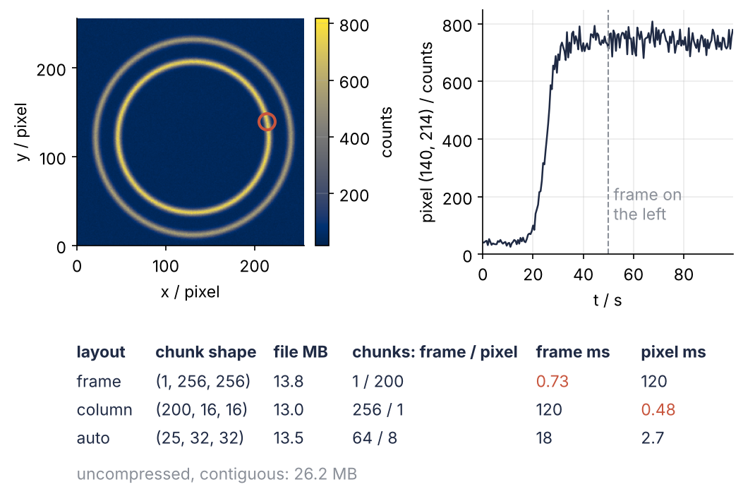
$Left: a simulated detector frame at 50 s, counts in color over x and y in pixels, two diffraction rings, one pixel circled. Right: its counts against time in s, jumping near 25 s as a new ring grows. Below: file size and read times of three chunk layouts, the cheapest read of each kind highlighted.$

This is where the page ends up: one frame read from the file, the history of one pixel on the growing ring, and what three ways of storing the same frames cost. A chunk per frame and a chunk per column of 16 × 16 pixels through all frames each make their own read take under a millisecond and the other read two orders of magnitude longer, while h5py's automatic choice sits in between.

Setup

The block below plays the detector: a seeded generator draws Poisson counts around three rings whose brightness changes at 25 s. From Step 1 on, the frames go to disk and come back from there. json, datetime, and platform serve only the record of the timings in Step 5.

import os
import json
import time
import datetime
import platform

import numpy as np
import h5py
import matplotlib.pyplot as plt

plt.rcParams.update({
    "figure.figsize": (8, 6.2), "figure.dpi": 110,
    "axes.spines.top": False, "axes.spines.right": False,
    "axes.grid": True, "grid.alpha": 0.25,
    "font.size": 11, "lines.linewidth": 1.8,
})
INK, ACCENT, SECOND, MUTED = "#1f2a44", "#c8553d", "#2a7f9e", "#8a8f98"

N_FRAMES, NY, NX = 200, 256, 256
DT = 0.5              # s between frames
EXPOSURE = 0.1        # s per frame
WAVELENGTH = 0.4133   # angstrom, 30 keV X-rays

rng = np.random.default_rng(20261009)
t = DT * np.arange(N_FRAMES)
y, x = np.mgrid[0:NY, 0:NX]
r = np.hypot(x - 131.0, y - 122.0)                       # distance from the beam center in pixels
ring = lambda radius: np.exp(-0.5 * ((r - radius) / 2.5) ** 2)
switch = 1 / (1 + np.exp(-(t - 25.0) / 2.0))[:, None, None]  # 0 before the transition, 1 after
mean = 40 + 600 * (1 - switch) * ring(60) + 700 * switch * ring(85) + 500 * ring(110)
frames = rng.poisson(mean).astype(np.uint16)

print(frames.shape, frames.dtype, f"{frames.nbytes / 1e6:.1f} MB")

(200, 256, 256) uint16 26.2 MB

Step 1: Write an array to a file with h5py.File and create_dataset

h5py.File opens a file in a mode: "w" creates it and empties it if it exists, "r" reads, "a" reads and writes and creates the file if needed. Use it in a with block, which closes the file at the end. Closing is what completes the file on disk; the pitfalls come back to that. Inside, create_dataset writes an array under a name:

with h5py.File("experiment.h5", "w") as f:
    f.create_dataset("frames", data=frames)

with h5py.File("experiment.h5", "r") as f:
    print(f["frames"])

size = os.path.getsize("experiment.h5")
print(f"file {size:,} bytes, array {frames.nbytes:,} bytes, {size - frames.nbytes:,} bytes more")

<HDF5 dataset "frames": shape (200, 256, 256), type "<u2">
file 26,216,448 bytes, array 26,214,400 bytes, 2,048 bytes more

The dataset knows its shape and its type, <u2, a little-endian unsigned 2-byte integer, which is NumPy's uint16. The file is the array plus 2,048 bytes of bookkeeping. HDF5 by itself adds almost nothing.

To fill a dataset later, frame by frame, give create_dataset a shape= and a dtype= instead of data=. It reserves the space, and you assign slices to it as to a NumPy array.

Step 2: Put datasets in groups and attach units as attributes

The file of Step 1 holds pixels and nothing else. Mode "w" replaces it with a tree. One convention carries through: every number is a dataset, a single value as a dataset with no axes, and next to it sits a units attribute; descriptions in words are attributes of a group or of the file. That is the NeXus convention in miniature. A group comes from create_group, or appears on its own when a dataset's name is a path such as "beam/wavelength":

with h5py.File("experiment.h5", "w") as f:
    f.attrs["title"] = "In-situ powder diffraction through a phase transition"
    f.attrs["created"] = "2026-10-09T14:00:00"

    detector = f.create_group("detector")
    detector.create_dataset("frames", data=frames).attrs["units"] = "counts"
    detector.create_dataset("exposure_time", data=EXPOSURE).attrs["units"] = "s"

    f.create_dataset("time", data=t).attrs["units"] = "s"
    f.create_dataset("beam/wavelength", data=WAVELENGTH).attrs["units"] = "angstrom"

    sample = f.create_group("sample")
    sample.attrs["name"] = "simulated powder"
    sample.attrs["description"] = "heated through a phase transition at t = 25 s"

To see what is in a file, visititems calls a function you give it once for every group and dataset, with the object's path and the object:

def show(path, obj):
    name = "    " * path.count("/") + path.split("/")[-1]
    kind = f"dataset {obj.shape} {obj.dtype}" if isinstance(obj, h5py.Dataset) else "group"
    attrs = "  ".join(f"{key}={value!r}" for key, value in obj.attrs.items())
    print(f"{name:18s} {kind:31s} {attrs}")

with h5py.File("experiment.h5", "r") as f:
    print(dict(f.attrs))
    f.visititems(show)

{'created': '2026-10-09T14:00:00', 'title': 'In-situ powder diffraction through a phase transition'}
beam               group                           
    wavelength     dataset () float64              units='angstrom'
detector           group                           
    exposure_time  dataset () float64              units='s'
    frames         dataset (200, 256, 256) uint16  units='counts'
sample             group                           description='heated through a phase transition at t = 25 s'  name='simulated powder'
time               dataset (200,) float64          units='s'

The wavelength has shape (), a single value. Someone who opens this file in ten years, in any language, does not need your notes to read it.

Step 3: Read one frame and one pixel without loading the file

Opening a dataset reads nothing. f["detector/frames"] is a handle that knows shape, type, and where the bytes are; data moves only when you slice it. Frame 100 is one slice, and the history of the pixel at row 140, column 214, which sits on the growing ring, is another:

with h5py.File("experiment.h5", "r") as f:
    dset = f["detector/frames"]
    print(type(dset).__name__, dset.shape, dset.dtype)
    frame = dset[100]
    series = dset[:, 140, 214]
    exposure = f["detector/exposure_time"]
    print(f"exposure time {exposure[()]} {exposure.attrs['units']}")

print(f"frame  {frame.shape}, {frame.nbytes:,} bytes, equal to the original: {np.array_equal(frame, frames[100])}")
print(f"series {series.shape}, {series.nbytes:,} bytes, every 40th value: {series[::40]}")

Dataset (200, 256, 256) uint16
exposure time 0.1 s
frame  (256, 256), 131,072 bytes, equal to the original: True
series (200,), 400 bytes, every 40th value: [ 41 100 733 753 727]

The frame comes back bit for bit, and the arrays are as small as the slices: 131 kB for a frame, 400 bytes for a pixel. How much the file has to read to deliver them is another number, and Step 4 counts it. The pixel sits at the background of 40 counts until the new ring appears, then at about 740.

The exposure time is read with [()], the empty index. It means "everything, no index", so on a dataset without axes it returns the one value, and on frames it would return all 26 MB.

How fast each read is depends on where the bytes lie. Without chunks, the frames sit on disk one after another in C order, row by row with the last index fastest, NumPy's default. A frame is then one contiguous run of bytes, while the pixel series is 200 values 131 kB apart. Chunks change that, and their shape is fixed when the dataset is created.

Step 4: Choose a chunk shape and compress with gzip

A chunked dataset is cut into blocks of one fixed shape. Each block is stored and compressed on its own, and it is read whole or not at all: a slice costs every chunk it touches, decompressed in full, not just its own bytes. Keep a chunk between about 10 kB and 1 MB: smaller, and the bookkeeping for each chunk dominates; larger, and every small read decompresses far more than it needs. h5py's own choice never exceeds 1 MiB, 2²⁰ bytes.

Three layouts of the same frames: a chunk per frame, a chunk per 16 × 16 column of pixels through all 200 frames, and h5py's guess with chunks=True. All three use compression="gzip" at its default level, 4. To count what a read costs, two helpers. np.s_[...] turns the slicing you would write inside brackets into an object you can pass to a function. dset.iter_chunks(selection) yields one entry for each chunk the selection touches, so counting the entries counts the chunks a read has to decompress:

LAYOUTS = {"frame": (1, NY, NX), "column": (N_FRAMES, 16, 16), "auto": True}
READS = {"frame": np.s_[100, :, :], "pixel": np.s_[:, 140, 214]}

print("layout  chunk shape     chunk kB  file MB   chunks per read   MB decompressed")
print("                                            frame   pixel     frame   pixel")
for name, chunks in LAYOUTS.items():
    with h5py.File(f"layout-{name}.h5", "w") as f:
        f.create_dataset("frames", data=frames, chunks=chunks, compression="gzip")
    with h5py.File(f"layout-{name}.h5", "r") as f:
        dset = f["frames"]
        chunk_bytes = np.prod(dset.chunks) * dset.dtype.itemsize
        touched = [sum(1 for _ in dset.iter_chunks(sel)) for sel in READS.values()]
    file_mb = os.path.getsize(f"layout-{name}.h5") / 1e6
    print(f"{name:7s} {str(dset.chunks):15s} {chunk_bytes / 1e3:7.1f} {file_mb:8.2f}"
          f" {touched[0]:7d} {touched[1]:7d}   {touched[0] * chunk_bytes / 1e6:7.2f} {touched[1] * chunk_bytes / 1e6:7.2f}")

layout  chunk shape     chunk kB  file MB   chunks per read   MB decompressed
                                            frame   pixel     frame   pixel
frame   (1, 256, 256)     131.1    13.76       1     200      0.13   26.21
column  (200, 16, 16)     102.4    13.04     256       1     26.21    0.10
auto    (25, 32, 32)       51.2    13.54      64       8      3.28    0.41

Every layout cuts the file to about half of 26.2 MB. Not further, because the Poisson noise in the low bits of each count is random, and gzip cannot compress randomness. The costs mirror each other: the per-frame layout touches 1 chunk for a frame and 200 for a pixel, the column layout 256 and 1. Reading one pixel's history from the per-frame file decompresses all 26.2 MB. The automatic guess, (25, 32, 32), sits in between with 64 and 8.

Compression needs chunks. Pass compression= without chunks= and h5py picks a chunk shape itself.

Step 5: Time the two reads for each layout

A fair timing opens the file afresh for every read and reads a different frame or pixel each time. HDF5 keeps recently read chunks in memory, a chunk cache of 1 MiB per open dataset in HDF5 before version 2.0 and 8 MiB since, so rereading the same frame measures memory, not the file. The file also sits in the operating system's cache after writing: these are times for decompression and bookkeeping, not for the disk. Each number is the median of 10 reads.

The helper below serves this page, not you: it stores each median in timings.json and returns the stored value on the next run, so the page shows the same numbers on every rebuild. Copying the code, keep the loop in median_ms, drop the lines that read or write timings and TIMINGS, and return 1e3 * np.median(times).

TIMINGS = "timings.json"
if os.path.exists(TIMINGS):
    with open(TIMINGS) as f:
        timings = json.load(f)
else:
    timings = {"date": str(datetime.date.today()),
               "machine": f"{platform.machine()}, Python {platform.python_version()}, "
                          f"h5py {h5py.__version__}, HDF5 {h5py.version.hdf5_version}"}

def median_ms(path, read):
    label = f"{path} {read.__name__}"
    if label not in timings:                       # returns the STORED time if label is in timings.json
        times = []
        for k in range(10):
            with h5py.File(path, "r") as f:        # a fresh file, so an empty chunk cache
                dset = f["frames"]
                start = time.perf_counter()
                read(dset, k)
                times.append(time.perf_counter() - start)
        timings[label] = float(f"{1e3 * np.median(times):.2g}")
        with open(TIMINGS, "w") as f:
            json.dump(timings, f, indent=1)
    return timings[label]

def read_frame(dset, k):
    return dset[10 + 18 * k]               # a different frame each time

def read_pixel(dset, k):
    return dset[:, 140, 70 + 16 * k]       # a different pixel, in a different column chunk

ms = {name: [median_ms(f"layout-{name}.h5", read) for read in (read_frame, read_pixel)] for name in LAYOUTS}
print(f"measured {timings['date']} on {timings['machine']}")
print("layout   frame ms   pixel ms")
for name, (t_frame, t_pixel) in ms.items():
    print(f"{name:7s} {t_frame:9g} {t_pixel:10g}")

measured 2026-10-09 on x86_64, Python 3.12.3, h5py 3.16.0, HDF5 2.0.0
layout   frame ms   pixel ms
frame        0.73        120
column        120       0.48
auto           18        2.7

The per-frame and the column layout each do their own read in under a millisecond and the other in about a tenth of a second, two orders of magnitude apart. The automatic guess is never the best: it takes about 20 ms for a frame and 2 to 3 ms for a pixel.

Step 4 says why. For a frame it decompresses 3.3 MB, an eighth of what the column layout does, and for a pixel 0.41 MB, a sixty-fourth of what the per-frame layout does, and its times shrink accordingly. The times grow in proportion to the megabytes decompressed, a few milliseconds per MB on this machine. Your times will differ from run to run and from machine to machine. The chunk counts and the megabytes will not. Trust them; the times only confirm them.

A detector writes frame by frame, so per-frame chunks are the natural choice when the data are taken, and the analysis that wants time series pays for it. Choose the chunks for the read you do most, or chunks=True when both matter.

Step 6: Draw the frame, the pixel, and the cost table

Each read comes from the layout made for it: the frame from layout-frame.h5, the series from layout-column.h5. The time axis and the units come from experiment.h5, and the axis labels are built from the units attributes, which is what the metadata is for. The frame is drawn with the cividis colormap.

K, ROW, COL = 100, 140, 214
with h5py.File("layout-frame.h5", "r") as f:
    image = f["frames"][K]
with h5py.File("layout-column.h5", "r") as f:
    series = f["frames"][:, ROW, COL]
with h5py.File("experiment.h5", "r") as f:
    t_read, t_units = f["time"][:], f["time"].attrs["units"]
    c_units = f["detector/frames"].attrs["units"]

fig = plt.figure(figsize=(8, 5.6))
grid = fig.add_gridspec(2, 2, height_ratios=[1.9, 1], width_ratios=[1, 1.1], hspace=0.45, wspace=0.75)
ax_img, ax_ts = fig.add_subplot(grid[0, 0]), fig.add_subplot(grid[0, 1])
ax_tab = fig.add_subplot(grid[1, :])

im = ax_img.imshow(image, cmap="cividis", origin="lower")
ax_img.plot(COL, ROW, "o", ms=11, mfc="none", mec=ACCENT, mew=2)
ax_img.set(xlabel="x / pixel", ylabel="y / pixel", xticks=[0, 100, 200], yticks=[0, 100, 200])
ax_img.grid(False)
cax = ax_img.inset_axes([1.05, 0, 0.06, 1])            # a colorbar exactly as tall as the frame
fig.colorbar(im, cax=cax, label=c_units)

ax_ts.plot(t_read, series, color=INK, lw=1.2)
ax_ts.axvline(t_read[K], color=MUTED, ls="--", lw=1)
ax_ts.text(t_read[K] + 2, 120, "frame on\nthe left", color=MUTED)
ax_ts.set(xlabel=f"t / {t_units}", ylabel=f"pixel ({ROW}, {COL}) / {c_units}",
          xlim=(0, t_read[-1]), ylim=(0, None))

ax_tab.set_axis_off()
columns = ["layout", "chunk shape", "file MB", "chunks: frame / pixel", "frame ms", "pixel ms"]
xs = [0.0, 0.12, 0.30, 0.42, 0.70, 0.86]
best = [min(v[0] for v in ms.values()), min(v[1] for v in ms.values())]
for xc, head in zip(xs, columns):
    ax_tab.text(xc, 0.85, head, color=INK, weight="bold", transform=ax_tab.transAxes)
for row, name in enumerate(LAYOUTS):
    with h5py.File(f"layout-{name}.h5", "r") as f:
        dset = f["frames"]
        chunks = dset.chunks
        touched = [sum(1 for _ in dset.iter_chunks(sel)) for sel in READS.values()]
    cells = [name, str(chunks), f"{os.path.getsize(f'layout-{name}.h5') / 1e6:.1f}",
             f"{touched[0]} / {touched[1]}", f"{ms[name][0]:g}", f"{ms[name][1]:g}"]
    colors = [INK] * 4 + [ACCENT if ms[name][i] == best[i] else INK for i in (0, 1)]
    for xc, cell, color in zip(xs, cells, colors):
        ax_tab.text(xc, 0.62 - 0.22 * row, cell, color=color, transform=ax_tab.transAxes)
ax_tab.text(0.0, -0.1, f"uncompressed, contiguous: {frames.nbytes / 1e6:.1f} MB", color=MUTED,
            transform=ax_tab.transAxes)
plt.show()

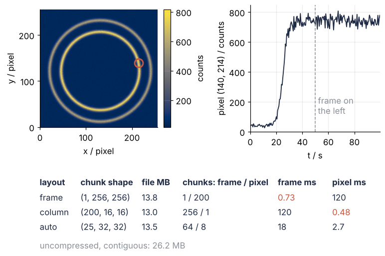
In the frame at 50 s the inner ring of the old phase is gone, and the series shows how long the new ring takes to grow in: about ten seconds, from 20 s to 30 s. The table puts Steps 4 and 5 side by side.

Pitfalls

Forgetting to close the file. Open with f = h5py.File("experiment.h5", "w") instead of a with block, run the cell a second time, and h5py answers OSError: Unable to synchronously create file (unable to truncate a file which is already open). The first handle still holds the file. Worse, HDF5 keeps part of the file in memory until it is closed, so another program that opens it meanwhile finds it incomplete. Use the with block, or call f.close() yourself; a file held by a handle you have lost is freed by restarting the kernel.

Python objects in attributes. An attribute holds a number, a string, or an array of them. A dictionary or None has no HDF5 type:

with h5py.File("scratch.h5", "w") as f:
    try:
        f.attrs["settings"] = {"gain": 2, "binning": 1}
    except TypeError as err:
        print(f"TypeError: {err}")
    f.attrs["settings"] = json.dumps({"gain": 2, "binning": 1})
    print(f.attrs["settings"])
os.remove("scratch.h5")

TypeError: Object dtype dtype('O') has no native HDF5 equivalent
{"gain": 2, "binning": 1}

Store one attribute per value, or turn a structure into a JSON string with json.dumps and back with json.loads.

Reading everything without meaning to. dset[:], dset[()], and np.array(dset) all read the whole dataset, and so does a function that receives the handle and converts it. Here that is 26 MB; for a real run it is more than your memory. Slice as in Step 3, and process a large dataset one frame at a time, for k in range(dset.shape[0]): process(dset[k]), which with per-frame chunks decompresses one chunk at a time.

Variations

Frames that arrive one by one. Create the dataset empty and extendable, create_dataset("frames", shape=(0, 256, 256), maxshape=(None, 256, 256), chunks=(1, 256, 256), dtype="u2"), then for each new frame dset.resize(n + 1, axis=0) and dset[n] = frame. An extendable dataset is always chunked.
The same file in Julia or on the command line. h5dump -H experiment.h5 prints the tree without the data. HDF5.jl opens the file with h5open and shows the frames with their axes reversed, (256, 256, 200), because Julia stores arrays column by column.
NeXus. The beamline standard is HDF5 with fixed group names and an NX_class attribute on every group (NXentry, NXdetector). The tree of Step 2 becomes /entry/instrument/detector/data.
A smaller file with the shuffle filter. Add shuffle=True next to compression="gzip". It stores the high bytes of all values together and the low bytes together, so gzip sees long runs of near-zero high bytes. On these frames the per-frame file shrinks from 13.8 to 11.3 MB.

Cheat sheet

with h5py.File("data.h5", "w") as f:                    # "r" read, "a" read and write
    d = f.create_dataset("group/name", data=a,          # intermediate groups appear on their own
                         chunks=(1, 256, 256),          # or True; fixed at creation
                         compression="gzip")            # level 4 by default; needs chunks
    d.attrs["units"] = "s"                              # numbers, strings, arrays; not dicts
    f.create_group("sample").attrs["name"] = "..."
with h5py.File("data.h5", "r") as f:
    d = f["group/name"]                                 # a handle; nothing read yet
    d[k], d[:, i, j], d[()]                             # only these; d[()] everything, a scalar's value
    d.shape, d.dtype, d.chunks; f.visititems(print)