Memory layout of NumPy arrays: why one axis sums faster than the other

The question

Take a 4000 × 4000 array of float64: 16,000,000 numbers at 8 bytes each, as in Vectorizing loops with NumPy, so 128,000,000 bytes, as much as 244 microscope frames of 512 × 512 pixels at 2 bytes each, or one field on a fine simulation grid. Sum it with a Python loop over its 4000 rows a[i], then with a loop over its 4000 columns a[:, j]. Both loops add the same numbers, stored in the same memory layout; only the order of reading differs.

The cell builds the array from a seeded generator and prints the cache sizes of the machine that built this page. The helper best_time takes the minimum of repeated runs, as in Profiling with cProfile and timeit, and best_pair times two or more operations in alternation, so that a drift of the machine hits both alike. Times are kept in timings.json for five minutes; after that, or with the file deleted, the page measures your machine again.

Show code

import datetime, json, os, platform, timeit
from pathlib import Path
import numpy as np
import matplotlib.pyplot as plt

plt.rcParams.update({
    "figure.figsize": (7, 3.6), "figure.dpi": 110,
    "axes.spines.top": False, "axes.spines.right": False,
    "axes.grid": True, "grid.alpha": 0.25,
    "font.size": 11, "lines.linewidth": 1.8,
})
INK, ACCENT, SECOND, MUTED = "#1f2a44", "#c8553d", "#2a7f9e", "#8a8f98"

rng = np.random.default_rng(273)
a = rng.random((4000, 4000))              # the values do not matter, only the size

TIMINGS = "timings.json"
if os.path.exists(TIMINGS):
    timings = json.loads(Path(TIMINGS).read_text())
else:
    timings = {"date": str(datetime.date.today()),
               "machine": f"{platform.machine()}, {os.cpu_count()} cores, NumPy {np.__version__}"}

def best_time(label, func, number=1, repeat=5):
    # returns the STORED time if label is in timings.json: delete the file to measure again
    if label not in timings:
        timings[label] = float(f"{min(timeit.repeat(func, number=number, repeat=repeat)) / number:.3g}")
        Path(TIMINGS).write_text(json.dumps(timings, indent=1))
    return timings[label]

def best_pair(labels, funcs, repeat=15):
    # timed in alternation, since a shared machine drifts by tens of percent between minutes
    if not all(label in timings for label in labels):
        runs = [[timeit.timeit(f, number=1) for f in funcs] for _ in range(repeat)]
        for label, ts in zip(labels, zip(*runs)):
            timings[label] = float(f"{min(ts):.3g}")
        Path(TIMINGS).write_text(json.dumps(timings, indent=1))
    return [timings[label] for label in labels]

def cache_sizes():
    """Data cache sizes in bytes by level, as Linux reports them; empty elsewhere."""
    sizes = {}
    try:
        for d in sorted(Path("/sys/devices/system/cpu/cpu0/cache").glob("index*")):
            if (d / "type").read_text().strip() in ("Data", "Unified"):
                sizes[int((d / "level").read_text())] = int((d / "size").read_text().strip().rstrip("K")) * 1024
    except OSError:
        pass
    return sizes

caches = cache_sizes()
print(f"a: {a.shape[0]} x {a.shape[1]} float64, {a.nbytes:,} bytes = {a.nbytes / 2**20:.0f} MiB")
print("caches: " + ("   ".join(f"L{k} {v / 2**10:,.0f} KiB" for k, v in caches.items()) or "unknown"))
print(f"timings measured {timings['date']} on {timings['machine']}")

a: 4000 x 4000 float64, 128,000,000 bytes = 122 MiB
caches: L1 32 KiB   L2 1,024 KiB   L3 33,792 KiB
timings measured 2026-10-10 on x86_64, 4 cores, NumPy 2.4.3

Four measurements: the two loops, and for comparison a copy of the array and a copy of its transpose.

Show code

def row_loop(a):
    return sum(a[i].sum() for i in range(a.shape[0]))          # 4000 row slices

def col_loop(a):
    return sum(a[:, j].sum() for j in range(a.shape[1]))       # 4000 column slices

t_row, t_col = best_pair(["row loop", "column loop"], [lambda: row_loop(a), lambda: col_loop(a)], repeat=5)
t_copy, t_tcopy = best_pair(["a.copy()", "a.T.copy()"], [lambda: a.copy(), lambda: a.T.copy()], repeat=9)
total_rows, total_cols = row_loop(a), col_loop(a)

print(f"sum over rows     {1e3 * t_row:4.0f} ms")
print(f"sum over columns  {1e3 * t_col:4.0f} ms   {t_col / t_row:.0f} times the rows")
print(f"a.copy()          {1e3 * t_copy:4.0f} ms")
print(f"a.T.copy()        {1e3 * t_tcopy:4.0f} ms   {t_tcopy / t_copy:.0f} times a.copy()")
print(f"the two sums: {total_rows:,.3f} and {total_cols:,.3f}, "
      f"relative difference {abs(total_rows - total_cols) / total_rows:.1e}")

fig, ax = plt.subplots(figsize=(7, 3))
labels = ["sum, rows  a[i]", "sum, columns  a[:, j]", "a.copy()", "a.T.copy()"]
times = np.array([t_row, t_col, t_copy, t_tcopy]) * 1e3
ypos = [3.2, 2.2, 0.9, -0.1]
ax.barh(ypos, times, height=0.75, color=[INK, ACCENT, INK, ACCENT])
for y, t, ratio in [(ypos[1], times[1], t_col / t_row), (ypos[3], times[3], t_tcopy / t_copy)]:
    ax.text(t + 2, y, f"{ratio:.0f} ×", va="center", color=ACCENT)
ax.set(yticks=ypos, yticklabels=labels, xlabel="time / ms", xlim=(0, 1.15 * times.max()))
ax.grid(axis="y", visible=False)
plt.show()

sum over rows       21 ms
sum over columns   167 ms   8 times the rows
a.copy()            34 ms
a.T.copy()         167 ms   5 times a.copy()
the two sums: 8,000,907.970 and 8,000,907.970, relative difference 3.3e-15

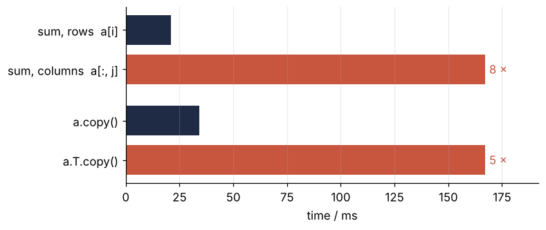
Time in ms of four operations on a 4000 by 4000 float64 array. Summing over column slices takes seven to ten times as long as over row slices; a.T.copy() takes three to six times as long as a.copy().

The obvious part holds: the two totals agree to a relative 3.3e-15, the rounding you get from adding in another order. The loop over columns takes about seven to ten times as long, depending on the run; the bar gives the factor this page measured. Copying shows the same split: a.T.copy() takes three to six times as long as a.copy(), although a.T by itself moves no number at all.

So the question is: why does the direction in which you read an array change the time by a factor of seven to ten, and how can you tell in advance which direction is the fast one?

The idea: a 2D array is a line of numbers with strides

Memory is one long line of bytes, each with a number, its address. There is no second dimension in it. NumPy puts the 16,000,000 numbers of a one after another on that line, row 0 first, then row 1, and so on. What makes them a 4000 × 4000 array is a small record kept next to the data: the address of the first number, and for each axis the number of bytes to step to reach the next index along it. These step sizes are the strides, and NumPy shows them as .strides.

Here is a 3 × 4 array with its strides, the strides of its transpose, and the strides of a:

Show code

small = np.arange(12.0).reshape(3, 4)
print(small)
print(f"small.strides   = {small.strides}")
print(f"small.T.strides = {small.T.strides}")
print(f"a.strides       = {a.strides}")

def offsets(view, i):
    """Positions on the memory line, in numbers, of row i of a view of small."""
    return [(i * view.strides[0] + j * view.strides[1]) // view.itemsize for j in range(view.shape[1])]

fig, axes = plt.subplots(2, 1, figsize=(7.5, 3.6), sharex=True)
for ax, view, name, color in [(axes[0], small, "small[1, :]", INK), (axes[1], small.T, "small.T[1, :]", ACCENT)]:
    hit = offsets(view, 1)
    for k in range(small.size):
        on = k in hit
        ax.add_patch(plt.Rectangle((k, 0), 0.92, 0.92, color=color if on else MUTED, alpha=0.9 if on else 0.2, lw=0))
        ax.text(k + 0.46, 0.46, f"{small.ravel()[k]:.0f}", ha="center", va="center",
                color="white" if on else INK)
    for p, q in zip(hit[:-1], hit[1:]):
        ax.annotate("", xy=(q + 0.46, 1.0), xytext=(p + 0.46, 1.0),
                    arrowprops=dict(arrowstyle="->", color=color, lw=1.2, connectionstyle="arc3,rad=-0.45"))
    step = view.strides[1]
    ax.text((hit[0] + hit[1]) / 2 + 0.46, 1.25 + 0.12 * (hit[1] - hit[0]), f"{step} B", ha="center", color=color)
    ax.text(-0.3, 0.46, name, ha="right", va="center", color=color)
    ax.set_axis_off()
    ax.set(xlim=(-3.2, small.size + 0.1), ylim=(-0.2, 2.0))
axes[1].text(small.size / 2, -0.15, "memory: 12 numbers of 8 bytes, one after another", ha="center", va="top", color=MUTED)
plt.show()

[[ 0.  1.  2.  3.]
 [ 4.  5.  6.  7.]
 [ 8.  9. 10. 11.]]
small.strides   = (32, 8)
small.T.strides = (8, 32)
a.strides       = (32000, 8)

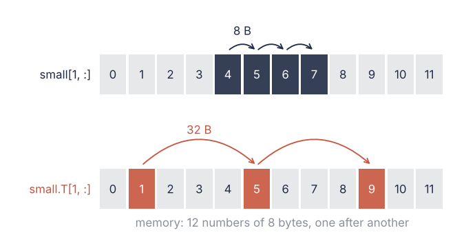
The 12 numbers of a 3 by 4 array on one memory line. A row of the array is four neighboring cells, 8 bytes apart; a row of its transpose is every fourth cell, 32 bytes apart.

To go from small[1, 0] to small[1, 1], NumPy steps 8 bytes, to the next number on the line. To go from small[0, 1] to small[1, 1], it steps 32 bytes, past a whole row of four. The transpose is the same 12 numbers on the same line, read with the two strides swapped, (8, 32). In the picture, a row of small is four neighbors, and a row of small.T, which is a column of small, is every fourth number. Nothing moves when you write small.T, which is why it is free.

For the big array the strides are (32000, 8). A row slice a[i] walks the line in steps of 8 bytes. A column slice a[:, j] jumps 32,000 bytes from one number to the next and touches 4000 places spread over all 128 MB. The arithmetic is the same; the walk is not.

Why reading across the line is slow: cache lines

The processor never fetches a single number from memory. It fetches the 64 bytes around it, a cache line, which holds 8 float64. When it sees a walk along memory in small regular steps, it also fetches the next lines before they are asked for, which is called prefetching.

Fetched lines are kept in caches, a ladder of small stores next to the processor, each larger and slower than the one before, with main memory larger and slower than all of them. On the machine that built this page the three levels, L1 to L3, hold 32 KiB, 1 MiB, and 33 MiB, as the first cell printed. Cache sizes come in KiB and MiB, 1024 and 1024² bytes; strides on this page stay in plain bytes. The array's 128,000,000 bytes are 122 MiB, so it lives in main memory, and every one of its lines has to come from there at least once.

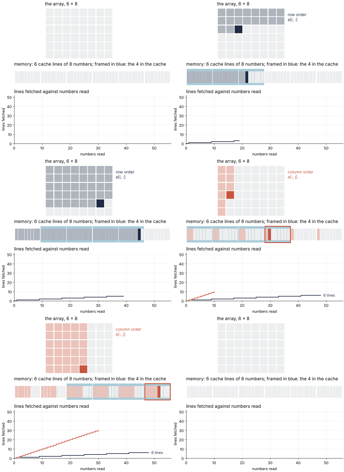
Along a row, one fetch serves 8 numbers. Down a column, one fetch serves one number. The other 7 on that line belong to the next 7 columns, and they help only if the line is still in a cache when the loop comes back for the next column. Here is that on a 6 × 8 array whose rows are one cache line each, read through a cache that holds 4 lines and throws out the one unused for longest:

A 6 by 8 array read in row order, then in column order, through a cache of 4 lines that evicts the least recently used. Watch the bottom panel: row order fetches 6 lines for 48 numbers, column order 48, one per number.

Show code

"""Cache walk: reading a 6 x 8 array by rows and by columns through a cache of 4 lines.

Renders ../../assets/cache-walk.gif. Run it from any directory:

    python scene.py
"""
from collections import OrderedDict
from pathlib import Path

import numpy as np
import matplotlib.pyplot as plt
from matplotlib.animation import FuncAnimation, PillowWriter
from matplotlib.patches import Rectangle
from PIL import Image

OUT = Path(__file__).resolve().parents[2] / "assets" / "cache-walk.gif"
INK, ACCENT, SECOND, MUTED = "#1f2a44", "#c8553d", "#2a7f9e", "#8a8f98"
plt.rcParams.update({"axes.spines.top": False, "axes.spines.right": False,
                     "axes.grid": True, "grid.alpha": 0.25, "font.size": 11})

ROWS, COLS, LINE, CACHE = 6, 8, 8, 4          # a row is one cache line of 8 numbers here


# ---- the walk: for each read, the element, the line it lives on, and whether it was fetched
def walk(order):
    cache = OrderedDict()                     # least recently used first
    reads, fetched = [], 0
    cells = [(i, j) for i in range(ROWS) for j in range(COLS)] if order == "row" else \
            [(i, j) for j in range(COLS) for i in range(ROWS)]
    for i, j in cells:
        line = (i * COLS + j) // LINE
        miss = line not in cache
        if miss:
            fetched += 1
            if len(cache) == CACHE:
                cache.popitem(last=False)     # evict the line unused for longest
        cache[line] = True
        cache.move_to_end(line)
        reads.append((i, j, line, miss, fetched, list(cache)))
    return reads


steps = {"row": walk("row"), "col": walk("col")}
color = {"row": INK, "col": ACCENT}
# frame list: (order, number of reads done); a blank frame at both ends closes the loop
frames = [(None, 0)] + [("row", k) for k in range(1, 49)] + [("row", 48)] * 6 \
         + [("col", k) for k in range(1, 49)] + [("col", 48)] * 8 + [(None, 0)]

# ---- figure, drawn once
fig, (ax1, ax2, ax3) = plt.subplots(3, 1, figsize=(7, 6.4), dpi=80, height_ratios=[1.5, 0.55, 1.4],
                                    layout="constrained")
array_cells = {(i, j): Rectangle((j, ROWS - 1 - i), 0.92, 0.92, color=MUTED, alpha=0.15, lw=0)
               for i in range(ROWS) for j in range(COLS)}
memory_cells = [Rectangle((k + 0.3 * (k // LINE), 0), 0.92, 0.92, color=MUTED, alpha=0.15, lw=0)
                for k in range(ROWS * COLS)]
held = [Rectangle((l * LINE + 0.3 * l - 0.12, -0.18), LINE + 0.16, 1.28, color=SECOND, alpha=0.0, lw=0)
        for l in range(ROWS)]
flash = Rectangle((0, -0.18), LINE + 0.16, 1.28, fill=False, ec=ACCENT, lw=2.5, visible=False)
# white cells under the memory cells, so the cache shading shows as a frame around them, not a tint
backing = [Rectangle(p.get_xy(), 0.92, 0.92, color="white", lw=0) for p in memory_cells]
for p in list(array_cells.values()):
    ax1.add_patch(p)
for p in held + backing + memory_cells + [flash]:
    ax2.add_patch(p)
order_text = ax1.text(COLS + 0.3, ROWS - 0.5, "", va="top", fontsize=12)
for ax in (ax1, ax2):
    ax.set_axis_off()
ax1.set(xlim=(-0.1, COLS + 3.2), ylim=(-0.1, ROWS + 0.05), aspect="equal")
ax2.set(xlim=(-0.3, ROWS * COLS + 0.3 * ROWS), ylim=(-0.3, 1.2))
ax1.set_title("the array, 6 × 8", loc="left")
ax2.set_title("memory: 6 cache lines of 8 numbers; framed in blue: the 4 in the cache", loc="left")
ax3.set_title("lines fetched against numbers read", loc="left")
curves = {o: ax3.plot([], [], color=color[o], lw=1.8, drawstyle="steps-post")[0] for o in steps}
counts = {o: ax3.text(49, 0, "", color=color[o], va="center") for o in steps}
ax3.set(xlim=(0, 56), ylim=(0, 52), xlabel="numbers read", ylabel="lines fetched")


# ---- one frame: the state after k reads in the given order
def update(frame):
    order, k = frame
    for o in steps:                                   # the row walk stays on the plot during the column walk
        done = 0 if order is None or (o == "col" and order == "row") else (k if o == order else 48)
        fetched = [0] + [s[4] for s in steps[o][:done]]
        curves[o].set_data(range(done + 1), fetched)
        counts[o].set_text(f"{fetched[-1]} lines" if done == 48 else "")
        counts[o].set_y(fetched[-1])
    for p in array_cells.values():
        p.set(color=MUTED, alpha=0.15)
    for p in memory_cells:
        p.set(color=MUTED, alpha=0.15)
    for p in held:
        p.set_alpha(0.0)
    flash.set_visible(False)
    order_text.set_text({"row": "row order\na[i, :]", "col": "column order\na[:, j]", None: ""}[order])
    order_text.set_color(color.get(order, INK))
    if order is None:
        return
    for i, j, line, miss, fetched, cache in steps[order][:k]:
        array_cells[i, j].set(color=color[order], alpha=0.35)
        memory_cells[i * COLS + j].set(color=color[order], alpha=0.35)
    i, j, line, miss, fetched, cache = steps[order][k - 1]
    array_cells[i, j].set_alpha(1.0)                  # the number being read now
    memory_cells[i * COLS + j].set_alpha(1.0)
    for l in cache:
        held[l].set_alpha(0.4)
    if miss and frames.count(frame) == 1:             # flash only on the read that fetched
        flash.set_x(line * LINE + 0.3 * line - 0.12)
        flash.set_visible(True)


# ---- render, and read back what was written
OUT.parent.mkdir(exist_ok=True)
FuncAnimation(fig, update, frames=frames).save(OUT, writer=PillowWriter(fps=12))
plt.close(fig)
with Image.open(OUT) as im:                           # Pillow merges repeated frames into longer ones
    total = 0
    for k in range(im.n_frames):
        im.seek(k)
        total += im.info["duration"]
    print(f"{OUT.name}: {im.width} x {im.height} px, {im.n_frames} stored frames, "
          f"{total / 1000:.1f} s, {OUT.stat().st_size / 1024:,.0f} kB")
print("lines fetched:", {o: s[-1][4] for o, s in steps.items()})

In row order the count of fetched lines ends at 6 for 48 numbers. In column order it ends at 48: each column needs all 6 lines, the cache holds 4, and the line needed next is always one that was just thrown out. So the factor 8 is a count, lines fetched per number read. Whether a real column loop pays all of it depends on whether some cache keeps one column's lines until the next column comes, and that can be measured.

Formalization

For an array with \(d\) axes and strides \(s_0, \dots, s_{d-1}\), the element with indices \((i_0, \dots, i_{d-1})\) sits at

\[\text{offset} = \sum_{k=0}^{d-1} i_k\, s_k\]

bytes from the first element. Every NumPy array is this formula plus a start address and an item size. An array is C-contiguous when its numbers fill a stretch of the line without gaps, last index fastest: the last stride equals the item size, and each earlier stride is the next one times the length of the next axis. It is Fortran-contiguous when the same holds with the axes taken in reverse, first index fastest. The names come from the default array layouts of the two programming languages. a.flags says which holds; a[::2] has a last stride of 8 bytes but skips every other row, so it is neither. Three consequences follow; the cell prints the strides, flags, and times this section quotes:

Show code

def shares(x):
    return np.shares_memory(a, x)

print("views: strides, and whether they share a's memory")
for name, v in [("a", a), ("a.T", a.T), ("a[:, ::2]", a[:, ::2]), ("a.reshape(-1)", a.reshape(-1)),
                ("a.ravel()", a.ravel())]:
    print(f"  {name:15s} strides {str(v.strides):14s} shares memory: {shares(v)}")
print(f"  a.flags['C_CONTIGUOUS'] = {a.flags['C_CONTIGUOUS']},  a.T.flags['F_CONTIGUOUS'] = {a.T.flags['F_CONTIGUOUS']}")
print(f"  a[::2] strides {a[::2].strides}:  C_CONTIGUOUS = {a[::2].flags['C_CONTIGUOUS']},  F_CONTIGUOUS = {a[::2].flags['F_CONTIGUOUS']}")

at = a.T
old = a[0, 1]
at[1, 0] = -1.0                       # write through the transposed view
print(f"after a.T[1, 0] = -1.0:  a[0, 1] = {a[0, 1]}")
a[0, 1] = old                         # and put the number back

print("copies")
for name, make in [("a.T.reshape(-1)", lambda: a.T.reshape(-1)), ("a.T.ravel()", lambda: a.T.ravel()),
                   ("a[a > 0.5]", lambda: a[a > 0.5]), ("a[[0, 2]]", lambda: a[[0, 2]])]:
    c = make()
    print(f"  {name:15s} shares memory: {shares(c)}")
    del c                             # a copy of a is up to 128 MB; free it at once

t_copy2, t_npcopy = best_pair(["a.copy(), next to np.copy", "np.copy(a.T)"], [lambda: a.copy(), lambda: np.copy(a.T)])
print(f"np.copy(a.T) {1e3 * t_npcopy:.0f} ms, a.copy() {1e3 * t_copy2:.0f} ms:  ratio {t_npcopy / t_copy2:.1f}")

total = a[0].copy()
for row in a[1:]:
    total += row                      # row after row, in memory order
print(f"a.sum(axis=0) equals adding row after row, to the last bit: {np.array_equal(total, a.sum(axis=0))}")
stack = a.reshape(250, 250, 256)      # the same bytes as a (t, y, x) stack of 250 frames
print("along t (axis=0) against along x (axis=2) of stack")
along_t = {}
for name, f in [("np.sum", np.sum), ("np.mean", np.mean), ("np.sort", np.sort),
                ("np.cumsum", np.cumsum), ("np.fft.rfft", np.fft.rfft)]:
    t_t, t_x = best_pair([f"{name}, t", f"{name}, x"], [lambda: f(stack, axis=0), lambda: f(stack, axis=2)], repeat=5)
    along_t[name] = t_t / t_x
    print(f"  {name:12s} {1e3 * t_t:4.0f} ms against {1e3 * t_x:4.0f} ms:  ratio {t_t / t_x:.0f}")

views: strides, and whether they share a's memory
  a               strides (32000, 8)     shares memory: True
  a.T             strides (8, 32000)     shares memory: True
  a[:, ::2]       strides (32000, 16)    shares memory: True
  a.reshape(-1)   strides (8,)           shares memory: True
  a.ravel()       strides (8,)           shares memory: True
  a.flags['C_CONTIGUOUS'] = True,  a.T.flags['F_CONTIGUOUS'] = True
  a[::2] strides (64000, 8):  C_CONTIGUOUS = False,  F_CONTIGUOUS = False
after a.T[1, 0] = -1.0:  a[0, 1] = -1.0
copies
  a.T.reshape(-1) shares memory: False
  a.T.ravel()     shares memory: False
  a[a > 0.5]      shares memory: False
  a[[0, 2]]       shares memory: False
np.copy(a.T) 32 ms, a.copy() 32 ms:  ratio 1.0
a.sum(axis=0) equals adding row after row, to the last bit: True
along t (axis=0) against along x (axis=2) of stack
  np.sum         15 ms against   15 ms:  ratio 1
  np.mean        13 ms against   13 ms:  ratio 1
  np.sort       177 ms against   79 ms:  ratio 2
  np.cumsum     174 ms against   65 ms:  ratio 3
  np.fft.rfft   159 ms against   77 ms:  ratio 2

Slices, transposes, and reshapes are views. A view is a new array that reads the bytes of another through its own start address and strides; making one copies nothing. a.T has strides (8, 32000) and a[:, ::2] has (32000, 16), and np.shares_memory says True for both. a is C-contiguous and a.T is Fortran-contiguous, one line seen two ways. Writing into a view writes into the original: setting a.T[1, 0] = -1.0 made a[0, 1] equal to -1.0. Indexing with a boolean mask or a list of indices, stack[mask] or a[[0, 2]], picks numbers no stride can describe, so it always returns a copy.

A column costs one cache line per number, unless lines are kept. A 64-byte line holds 8 float64, so reading a row by row fetches 2,000,000 lines, and column by column 16,000,000 if no line survives until the next column. To see where a real loop lands between the two, view the same 128 MB as rows of L numbers, a.reshape(-1, L), and read it column by column. Call one column of that view a pass: 16,000,000 / L numbers, 8L bytes apart, and the L passes together read every number once. The line count then predicts the time per number. It grows in proportion to the stride from 8 B to 64 B, since one line serves 64 / stride numbers of a pass, and stays flat beyond, at 8 times the contiguous read, as long as no line is kept from one pass to the next. It falls only where a pass is short, few numbers at a large stride, so that its lines stay in a cache until the next pass reads their neighbors. L = 4000 is the question's column loop: each pass touches 4000 lines, 250 KiB, which fits the 1 MiB L2 by size. Whether the lines are actually kept, only the measurement says.

Some reshapes and copies are hidden reorderings. a.reshape(-1) and a.ravel() return views, because a read in C order is the line itself. a.T.reshape(-1) and a.T.ravel() must copy, since the transposed order jumps 32,000 bytes and then back, which no single stride describes. a.T.copy() defaults to order="C", so one side of the copy, reading or writing, goes across the line: that is the factor of three to six in the question. np.copy(a.T) defaults to order="K", which keeps the input's layout, and takes about as long as a.copy(). When a loop will read a transposed array many times, np.ascontiguousarray(a.T) pays one reordering copy so that every later pass walks along the line.

None of this slows sum, mean, or max, because for these NumPy orders the loop by the strides itself. For a.sum(axis=0) it walks a in memory order and adds row after row into 4000 totals, as the cell confirms to the last bit. With the same bytes viewed as a (t, y, x) stack of 250 frames, stack.sum(axis=0) and stack.mean(axis=0) along t take the same time as along x. Other functions do pay. np.argmax along t first makes a copy of the whole stack, which it does not need along x. np.sort, np.cumsum, and np.fft.rfft, which take one 1D slice at a time, run two to three times longer along t than along x. So does a Python loop over slices across the line, as the question showed.

See it in code

The cell runs the sweep for 15 values of L, from 1 to 16,000, minus the microsecond or so of overhead per .sum() call. Next to it: the question's two loops, and one column summed 1000 times, a cache's best chance to keep it.

Show code

line = a.reshape(-1)                                  # the 16,000,000 numbers in memory order
assert np.shares_memory(line, a)
# The row loop is about half call overhead, so the overhead is timed as the same loop over
# one-number slices, in alternation with it: timed apart, it varied twofold from run to run.
t_row2, t_empty = best_pair(["row loop, next to its overhead", "loop over one-number slices"],
                            [lambda: row_loop(a), lambda: sum(a[i, :1].sum() for i in range(4000))], repeat=9)
t_call = t_empty / 4000

Ls = [1, 2, 4, 8, 16, 32, 64, 128, 256, 512, 1024, 2000, 4000, 8000, 16000]
views = [line.reshape(-1, L) for L in Ls]             # rows of L numbers: a column steps 8 L bytes
# all 15 timed in alternation, so that a drift of the machine moves the whole curve, not one point
t_sweep = np.array(best_pair([f"columns of {L}" for L in Ls],
                             [lambda v=v: sum(v[:, j].sum() for j in range(v.shape[1])) for v in views], repeat=5))
stride = np.array([v.strides[0] for v in views])
ns = (t_sweep - np.array(Ls) * t_call) / line.size * 1e9   # L calls of .sum(), each with its overhead
correction = np.array(Ls) * t_call / t_sweep
predicted = ns[0] * np.minimum(stride, 64) / 8        # one cache line per 64 / stride numbers

t_col_again = best_time("a[:, 0].sum() x1000", lambda: a[:, 0].sum(), number=1000)
t_row_again = best_time("a[0].sum() x1000", lambda: a[0].sum(), number=1000)
per_number = {"row loop": (t_row2 - t_empty) / a.size * 1e9,
              "column loop": (t_col - t_empty) / a.size * 1e9,
              "one column again": (t_col_again - t_call) / 4000 * 1e9}
row_again = (t_row_again - t_call) / 4000 * 1e9

print(f"one .sum() call costs {1e6 * t_call:.1f} µs, subtracted below: {100 * correction[-1]:.0f} % of the time "
      f"at {stride[-1]:,} B, {100 * correction[Ls.index(512)]:.1f} % at {stride[Ls.index(512)]:,} B")
print("stride / B   time per number / ns")
for s, n in zip(stride, ns):
    print(f"{s:10,d}   {n:6.2f}")
plateau = ns[(stride >= 128) & (stride <= 32_000)]
print(f"64 B over 8 B: {ns[3] / ns[0]:.0f}   128 B to 32,000 B over 64 B: {plateau.min() / ns[3]:.1f} to {plateau.max() / ns[3]:.1f}"
      f"   over the guide: {plateau.min() / predicted[-1]:.1f} to {plateau.max() / predicted[-1]:.1f}")
print("per number:  " + "   ".join(f"{k} {v:.2f} ns" for k, v in per_number.items())
      + f"   one row again {row_again:.2f} ns")
print(f"one column again over one new column in the loop: {per_number['one column again'] / per_number['column loop']:.2f}")

fig, (ax, bx) = plt.subplots(1, 2, figsize=(8, 3.6), sharey=True, gridspec_kw={"width_ratios": [2.6, 1.2]})
ax.plot(stride, predicted, color=MUTED, lw=1.2, ls="--")
ax.plot(stride, ns, "o-", color=ACCENT, ms=6)
ax.axvline(64, color=MUTED, lw=1, ls="--")
ax.text(70, 0.5, "cache line", color=MUTED)
# Labels sit where no re-measurement can reach: under the guide between 160 B and
# 32,000 B (the flat stretch stays above 0.85 of it), and above 15 ns (its ceiling).
ax.text(160, predicted[-1] * 0.75, "one line per number,\nnothing kept", color=MUTED, ha="left", va="top")
k = Ls.index(4000)
ax.annotate("the column loop", (stride[k], ns[k]), xytext=(stride[k] * 1.3, 16.5), textcoords="data",
            ha="right", va="bottom", color=ACCENT, arrowprops=dict(arrowstyle="-", color=ACCENT, lw=1, relpos=(1, 0)))
ticks = [8, 64, 512, 4096, 32_000]                          # plain bytes, as in the prose
ax.set(xscale="log", yscale="log", xticks=ticks, xticklabels=[f"{t:,}" for t in ticks],
       xlabel="stride of the access / bytes", ylabel="time per number / ns", ylim=(0.4, 25))
ax.set_yticks([0.5, 1, 2, 5, 10], ["0.5", "1", "2", "5", "10"])
ax.minorticks_off()
bar_colors = [INK, ACCENT, SECOND]
bx.bar(range(3), list(per_number.values()), color=bar_colors, width=0.7)
for x, (v, c) in enumerate(zip(per_number.values(), bar_colors)):
    bx.text(x, v * 1.08, f"{v:.1f}", ha="center", va="bottom", color=c)        # ns per number
bx.set(xticks=range(3), xticklabels=["row\nloop", "column\nloop", "same\ncolumn"])
bx.grid(axis="x", visible=False)
plt.show()

one .sum() call costs 1.8 µs, subtracted below: 42 % of the time at 128,000 B, 0.5 % at 4,096 B
stride / B   time per number / ns
         8     0.84
        16     1.60
        32     2.91
        64     5.62
       128    10.87
       256    11.00
       512     9.99
     1,024     9.67
     2,048    10.47
     4,096    11.26
     8,192    10.70
    16,000     9.78
    32,000     9.81
    64,000     5.15
   128,000     2.50
64 B over 8 B: 7   128 B to 32,000 B over 64 B: 1.7 to 2.0   over the guide: 1.4 to 1.7
per number:  row loop 0.93 ns   column loop 9.99 ns   one column again 9.03 ns   one row again 0.12 ns
one column again over one new column in the loop: 0.90

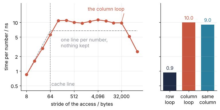
Left: time per number in ns against the stride in bytes, log scales. It rises to 64 B, stays flat at 7 to 15 ns up to 32,000 B, near or above a dashed one-line-per-number guide, and falls at 64,000 and 128,000 B. Right: row loop about 1 ns, column loop and repeated column about 10 ns.

Up to 64 B the time per number grows five- to eightfold, against 8 predicted. From 128 B to 32,000 B it is flat, as predicted, but above the 64 B point, where every number also costs one line. At 64 B a pass reads neighboring lines, which prefetching fetches ahead; beyond, it skips lines, and each costs more. The dashed guide prices each line at eight contiguous reads, and the flat stretch lies near or above it.

The third bar settles reuse: the same column again costs about as much per number as a new one. Its 250 KiB would fit the L2 and are not kept, so fitting by size is not a safe rule; the sweep falls only where a pass has 2000 numbers or fewer. Details beyond size decide: an address may go into only a few slots of a cache, prefetching does not follow long jumps, and each number of a column sits on its own memory page (the 4 KiB unit the operating system hands out), and the processor tracks only so many pages. Processors differ in all three; yours may place the fall elsewhere.

Where it shows up

The array in the question belongs to no field, and the same walk across the line turns up in all of them.

Biology: microscopy and calcium imaging. A stack stored as (t, y, x) puts each frame on the line, so stack.mean(axis=0) needs no help, while the time trace of one pixel, stack[:, y, x], steps one whole frame per value. Before traces are sorted or transformed one at a time, or read in a loop more than once, np.ascontiguousarray(stack.transpose(1, 2, 0)) makes a (y, x, t) copy in which every trace is contiguous.
Physics and engineering: finite-difference grids. An ADI solver for the heat equation alternates tridiagonal solves along one axis and then the other, and on a C-ordered grid the solves down the columns u[:, j] read across the line. One np.ascontiguousarray(u.T) between the half-steps makes both sweeps walk along it.
Geology: seismometer arrays. A recording stored as (time, station) and processed by a Python loop over stations, x[:, k], reads across the line once per station. Storing it as (station, time), or making it so once with np.ascontiguousarray(x.T), puts each station's trace on the line.
Chemistry: handing matrices to compiled libraries. LAPACK, the Fortran library under scipy.linalg, works on Fortran-ordered matrices, so scipy.linalg.eigh(H, overwrite_a=True) on a Hamiltonian or Fock matrix can only work in place when H is Fortran-contiguous. On a C-ordered H the flag changes nothing: the matrix is copied first, and H comes back untouched.

In each of them the cost comes from code that walks the array in an order of its own, a Python loop over slices or a compiled routine that expects one layout; a sum or mean over the whole array chooses its order itself and needs no copy.

The question

The idea: a 2D array is a line of numbers with strides

Why reading across the line is slow: cache lines

Formalization

See it in code

Where it shows up

Further reading