NetworkX from the ground up: the fault line through a karate club

The problem: who went with whom when the karate club split?

In the early 1970s the anthropologist Wayne Zachary studied a university karate club of about 60 members and recorded who spent time with whom outside the club: 34 members, joined by 78 friendships. While he watched, the club broke apart. A dispute between the instructor, whom the data call Mr. Hi, and the club's president, labeled Officer, split it in two. NetworkX ships the friendship network together with the side Zachary recorded for each of the 34 after the split, so the question can be put to the data. Do the friendships alone, without knowing who left with whom, show the fault line? And how many of the 34 end up on the wrong side of it?

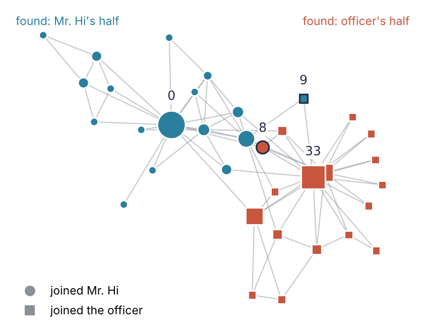
This is where we end up. Each marker is a member, each line a friendship. The color is the half that community detection finds from the friendships alone, the shape is the side the member actually joined, and the size is betweenness, defined in Step 4, which is large for a member that many shortest routes between others pass through. Color and shape disagree for 2 of the 34 members, nodes 8 and 9. The rest of this tutorial builds that figure.

Setup

The network ships with NetworkX, so there is nothing to download. It comes from Zachary's paper "An information flow model for conflict and fission in small groups", Journal of Anthropological Research 33, 452 (1977).

from collections import Counter

import matplotlib.pyplot as plt
import networkx as nx
import numpy as np

plt.rcParams.update({                      # the look of every figure below
    "figure.figsize": (7, 3.2), "figure.dpi": 110,
    "axes.spines.top": False, "axes.spines.right": False,
    "axes.grid": True, "grid.alpha": 0.25,
    "font.size": 11, "lines.linewidth": 1.8,
})
INK, ACCENT, SECOND, MUTED = "#1f2a44", "#c8553d", "#2a7f9e", "#8a8f98"
SEED = 0           # for community detection
LAYOUT_SEED = 3    # for the drawing; any value works, this one reads well

G = nx.karate_club_graph()
print(G)

Graph named "Zachary's Karate Club" with 34 nodes and 78 edges

Step 1: Look inside a graph: nodes, edges, and attributes

A Graph holds nodes, edges between pairs of nodes, and a dictionary of attributes on every node and every edge. You read them with square brackets, the way you read any dictionary:

print(G.nodes[0])
print(G.edges[0, 1])
print(list(G.neighbors(0))[:6])
print(Counter(nx.get_node_attributes(G, "club").values()))

{'club': 'Mr. Hi'}
{'weight': 4}
[1, 2, 3, 4, 5, 6]
Counter({'Mr. Hi': 17, 'Officer': 17})

Node 0 joined Mr. Hi, and 17 members went each way. The weight on an edge is Zachary's count of the contexts in which a pair met, from 1 to 7. This tutorial counts friendships, not contexts, so every function that reads weight by default gets weight=None: community detection, modularity, and the layout. The path and centrality functions ignore weights unless you ask.

Your own graph takes two lines. Any hashable object can be a node, and an edge attribute is a keyword argument:

H = nx.Graph([("C", "H1"), ("C", "H2")])   # straight from a list of pairs
H.add_edge("C", "O", order=2)             # adding an edge adds its nodes
print(H, H.edges["C", "O"])

Graph with 4 nodes and 3 edges {'order': 2}

That is formaldehyde, with the bond order on the double bond.

Step 2: Count degrees and plot the degree distribution

The degree of a node is its number of edges, here its number of friends. G.degree is a view of (node, degree) pairs, not a list, so sort it by the second entry:

Copy

print(sorted(G.degree, key=lambda pair: pair[1], reverse=True)[:5])
print(f"mean degree {2 * G.number_of_edges() / G.number_of_nodes():.2f}")   # each edge adds to two degrees
hist = nx.degree_histogram(G)           # hist[k] = number of nodes with degree k
print(hist)

k = np.arange(len(hist))
fig, ax = plt.subplots()
ax.bar(k, hist, width=0.8, color=INK)
ax.text(15.5, 0.5, "node 0", ha="right", va="center")      # names beside the two bars
ax.text(17.5, 0.5, "node 33", ha="left", va="center")
ax.set(xlabel="degree (number of friends)", ylabel="members", xticks=range(0, 20, 2), xlim=(-0.6, 19.8))
plt.show()

[(33, 17), (0, 16), (32, 12), (2, 10), (1, 9)]
mean degree 4.59
[0, 1, 11, 6, 6, 3, 2, 0, 0, 1, 1, 0, 1, 0, 0, 0, 1, 1]

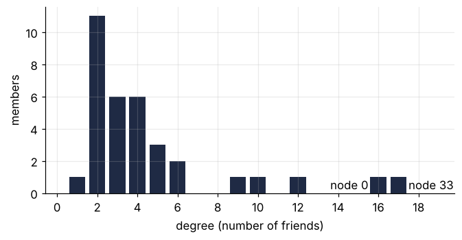
Nodes 33 and 0 have 17 and 16 friends, against a mean of 4.59. Most members have two to five friends, 11 of them exactly two. Two members have more than three times the mean, and before any centrality is computed they are the candidates for the two leaders.

Step 3: Measure distance: shortest paths and the diameter

A path is a chain of edges from one node to another, and its length is the number of edges. Distance in a network counts steps from friend to friend, not meters, the way a chemist counts the bonds between two atoms. A graph is connected when every node can reach every other, and its diameter is the largest distance between any pair. Start with the two members who have the most friends:

print(nx.shortest_path(G, 0, 33))
for path in nx.all_shortest_paths(G, 0, 33):
    print("   ", path)
print("connected:", nx.is_connected(G))
print(f"average distance {nx.average_shortest_path_length(G):.2f}, diameter {nx.diameter(G)}")

[0, 8, 33]
    [0, 8, 33]
    [0, 13, 33]
    [0, 19, 33]
    [0, 31, 33]
connected: True
average distance 2.41, diameter 5

shortest_path returns [0, 8, 33], but there are four shortest paths of length 2, through nodes 8, 13, 19, and 31, and the function hands you one of them without a word. When the choice matters, as it does for who connects two people, ask for all of them with all_shortest_paths. Two members are 2.41 steps apart on average and never more than 5. diameter and average_shortest_path_length raise an error on a graph that is not connected, which is why the check comes first.

Step 4: Rank the members by centrality: degree, betweenness, closeness

Centrality is a number per node that answers "who matters", and there is more than one answer. Degree centrality is the degree divided by 33, the most friends a member could have. Betweenness takes every pair of other members, finds the fraction of their shortest paths that pass through the node, and averages it over the pairs. Closeness is one over the mean distance to everyone else.

centrality = {
    "degree": nx.degree_centrality(G),
    "betweenness": nx.betweenness_centrality(G),
    "closeness": nx.closeness_centrality(G),
}
for name, c in centrality.items():
    top = sorted(c, key=c.get, reverse=True)[:5]
    print(f"{name:12s}" + "   ".join(f"{n:2d}: {c[n]:.3f}" for n in top))
print(G.nodes[0]["club"], G.nodes[33]["club"])

degree      33: 0.515    0: 0.485   32: 0.364    2: 0.303    1: 0.273
betweenness  0: 0.438   33: 0.304   32: 0.145    2: 0.144   31: 0.138
closeness    0: 0.569    2: 0.559   33: 0.550   31: 0.541    8: 0.516
Mr. Hi Officer

By degree node 33 leads, by betweenness node 0 leads clearly, 0.438 against 0.304. Node 31 has only six friends and still ranks fifth by betweenness, at 0.138. It is a broker, a member the shortest routes between groups run through, and degree cannot see that. Closeness separates the members less sharply: 0.569 for node 0 means 1.76 steps to the average member, and the top values crowd together because everyone is within a few steps of everyone. The last line shows the side each of the two joined. That they are the leaders themselves, node 0 the instructor and node 33 the president, comes from Zachary's paper, not from the data.

Step 5: Find communities with louvain_communities and choose the resolution

A community is a group of nodes with more edges among themselves than to the rest. louvain_communities finds them, given weight=None (Step 1) and a seed:

groups = nx.community.louvain_communities(G, weight=None, seed=SEED)
for g in sorted(groups, key=len):
    print(len(g), dict(Counter(G.nodes[n]["club"] for n in g)))

5 {'Mr. Hi': 5}
6 {'Officer': 6}
11 {'Mr. Hi': 11}
12 {'Officer': 11, 'Mr. Hi': 1}

Four groups, three from one side only. Louvain moves nodes between groups as long as a score called modularity rises, in a random order that the seed fixes.

Modularity \(Q\) is the fraction of edges inside the groups minus the fraction that would fall inside if the same degrees were wired at random. A group's expected share grows with the square of its total degree, so a big group catches more random edges. \(Q = 0\) means the groups are no denser than chance, and 1 is out of reach. Louvain maximizes

with \(\gamma\) the argument resolution. Below 1, big groups cost less, so merging pays. Every \(Q\) printed here is at \(\gamma = 1\), so splits compare on one scale.

To choose the resolution, scan it down from 1, 20 seeds per value, until every seed returns one group. A set of sets has no order, so the same split from two seeds compares equal and Counter can count it:

print("resolution   group counts seen   groups in top split   seeds behind it")
for r in range(10, 0, -1):
    resolution = r / 10
    splits = Counter(
        frozenset(frozenset(g) for g in nx.community.louvain_communities(
            G, weight=None, resolution=resolution, seed=s))
        for s in range(20)
    )
    best, n_seeds = splits.most_common(1)[0]
    seen = sorted({len(split) for split in splits})        # every number of groups some seed returned
    print(f"{resolution:10.1f}   {str(seen):17s}   {len(best):19d}   {n_seeds:9d} of 20")
    if len(best) == 1 and n_seeds == 20:
        break

resolution   group counts seen   groups in top split   seeds behind it
       1.0   [4]                                   4           6 of 20
       0.9   [3, 4]                                4           7 of 20
       0.8   [2, 3, 4]                             3          13 of 20
       0.7   [2, 3]                                3          13 of 20
       0.6   [2]                                   2          18 of 20
       0.5   [2]                                   2          19 of 20
       0.4   [2]                                   2          19 of 20
       0.3   [2]                                   2          18 of 20
       0.2   [1]                                   1          20 of 20

From 0.6 to 0.3 the same two-group split comes back from 18 or 19 of 20 seeds, and no split into three or four groups gets more than 13. The single group at 0.2 says nothing: it holds every edge and every expected edge, so its \(Q\) is 0.

The rule: drop the single group and keep the widest run on which the seeds agree far better than anywhere else in the table. Take a resolution from inside it. Here that gives two halves, found without Zachary's account:

halves = nx.community.louvain_communities(G, weight=None, resolution=0.5, seed=SEED)
inside = sum(G.subgraph(h).number_of_edges() for h in halves)   # edges with both ends in one half
print([len(h) for h in halves], f"{inside} of {G.number_of_edges()} edges inside",
      f"Q = {nx.community.modularity(G, halves, weight=None):.3f}")

splits = Counter(frozenset(frozenset(g) for g in nx.community.louvain_communities(G, weight=None, seed=s))
                 for s in range(20))                              # back to resolution 1
Q = [nx.community.modularity(G, split, weight=None) for split in splits]
print(f"resolution 1: {len(splits)} different splits, Q from {min(Q):.3f} to {max(Q):.3f}")
four = frozenset(frozenset(g) for g in groups)
print(f"the four groups from the first call: Q = {nx.community.modularity(G, groups, weight=None):.3f},",
      f"{splits[four]} of 20 seeds")

[17, 17] 68 of 78 edges inside Q = 0.372
resolution 1: 5 different splits, Q from 0.395 to 0.420
the four groups from the first call: Q = 0.420, 3 of 20 seeds

The halves score \(Q = 0.372\) and hold 0.872 of the friendships, against 0.500 by chance. At resolution 1 the seeds end in five splits with \(Q\) from 0.395 to 0.420, and the best, the first call's four groups, comes from only 3 of 20. Louvain stops once no move raises \(Q\), and the seed picks which of these near-equal splits that is. A split another seed would not return is not a finding, however high its \(Q\).

Step 6: Compare with the actual split and draw the network

Name each half by the leader it contains, node 0 or node 33 from Steps 2 and 4, and only now look at club. The cut of a split is the set of edges that cross between its halves:

hi = next(h for h in halves if 0 in h)                 # the half around the instructor
found = {n: "Mr. Hi" if n in hi else "Officer" for n in G}
wrong = [n for n in G if found[n] != G.nodes[n]["club"]]
print("on the wrong side:", wrong)
for n in wrong:
    print(n, dict(Counter(G.nodes[m]["club"] for m in G.neighbors(n))))

actual = [{n for n in G if G.nodes[n]["club"] == side} for side in ("Mr. Hi", "Officer")]
inside = sum(G.subgraph(h).number_of_edges() for h in actual)
print(f"actual split: {inside} edges inside, Q = {nx.community.modularity(G, actual, weight=None):.3f}")
print("cut:", nx.cut_size(G, hi), "found,", nx.cut_size(G, actual[0]), "actual")

on the wrong side: [8, 9]
8 {'Mr. Hi': 2, 'Officer': 3}
9 {'Mr. Hi': 1, 'Officer': 1}
actual split: 67 edges inside, Q = 0.358
cut: 10 found, 11 actual

Two of 34. Node 9 has one friend on each side. Node 8 has three of its five friends on the officer's side and went with Mr. Hi anyway. The actual split scores \(Q = 0.358\), with 67 friendships inside. Its cut has 11 edges against 10 for the split Louvain found, so the members' own line crosses one friendship more.

nx.spring_layout treats every edge as a spring that pulls its two nodes together while all nodes push one another apart, and moves the nodes from random starting positions until the forces nearly balance, hence the seed. Densely linked groups end up close together, but the axes have no units, and distance on the page follows distance in the network only roughly. The drawing functions take an ax, like every plot in Matplotlib from the ground up:

Copy

pos = nx.spring_layout(G, seed=LAYOUT_SEED, weight=None)   # node -> (x, y) array
btw = centrality["betweenness"]

fig, ax = plt.subplots(figsize=(7, 5.5))
nx.draw_networkx_edges(G, pos, ax=ax, edge_color=MUTED, alpha=0.5, width=1)
for side, shape in [("Mr. Hi", "o"), ("Officer", "s")]:     # one marker shape per call
    nodes = [n for n in G if G.nodes[n]["club"] == side]
    nx.draw_networkx_nodes(
        G, pos, nodelist=nodes, node_shape=shape, ax=ax,
        node_color=[SECOND if n in hi else ACCENT for n in nodes],
        node_size=[60 + 1500 * btw[n] for n in nodes],       # area grows with betweenness
        edgecolors=[INK if n in wrong else "white" for n in nodes], linewidths=1.5)   # the ring
nx.draw_networkx_labels(G, {n: pos[n] + (0, 0.07 + 0.1 * btw[n]) for n in (0, 33, 8, 9)},
                        labels={n: n for n in (0, 33, 8, 9)}, ax=ax, font_color=INK,
                        bbox=dict(fc="white", ec="none", pad=1))   # keeps edges off the numbers
ax.text(0.02, 0.98, "found: Mr. Hi's half", color=SECOND, transform=ax.transAxes, va="top")
ax.text(0.98, 0.98, "found: officer's half", color=ACCENT, transform=ax.transAxes, va="top", ha="right")
handles = [plt.Line2D([], [], ls="", marker=m, ms=9, color=MUTED, label=label)
           for m, label in [("o", "joined Mr. Hi"), ("s", "joined the officer")]]
ax.legend(handles=handles, frameon=False, loc="lower left")
ax.set_axis_off()
plt.show()

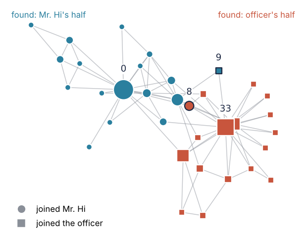
The two large nodes anchor the two halves. Nodes 8 and 9, ringed, sit between the groups, where the springs from both sides pull on them.

Pitfalls

An unseeded layout or community search. The picture rearranges on every run, and Louvain returns different groups: five different splits from 20 seeds at the default resolution. Both are random searches, as Step 5's scan and Step 6's springs showed. Pass seed= to louvain_communities and to spring_layout, and trust a split only after a scan like Step 5's, never after one lucky seed. A new layout seed rotates or mirrors the picture and moves a few nodes, but the groups stay together.

Reading meaning into node numbers. The numbers are labels. NetworkX counts from 0 and Zachary from 1, so NetworkX's node 33 is his member 34, and the misassigned 8 and 9 are his members 9 and 10. That matters the moment you compare with a paper. Add 1 before you compare, or relabel once with nx.relabel_nodes(G, lambda n: n + 1), which changes no result. Neighboring numbers say nothing about neighbors.

Drawing a large network as a hairball. A network of 34 nodes draws well. A thousand nodes in a spring layout give a gray ball that shows nothing but its own outline. Look at the degree histogram, the diameter, and the community sizes first, and when you want a picture, draw a subgraph: one community with G.subgraph(nodes), or nx.ego_graph(G, n), which returns node n, its neighbors, and the edges among them.

Variations

• The weighted network. Drop weight=None, and Louvain and modularity read Zachary's counts as the strength of a tie. At resolution=0.5 and seed 0 only node 8 stays on the wrong side. Shortest paths and betweenness read a weight as a length and spring_layout as the stiffness of a spring, so for paths store 1 / weight as a new edge attribute and pass its name.
• A null model. nx.double_edge_swap on a seeded copy rewires the edges while every node keeps its degree. Run Louvain on many copies and compare their modularity with the 0.420 of the four groups. The copies do not score zero, because a search for the best split finds some structure in any graph.
• Spreading on the network. An SIR epidemic: at each step every infected node infects each susceptible neighbor with probability \(\beta\) and recovers with probability \(\mu\), with draws from one generator of Random numbers with numpy.random. Start at a leader, then at a member on the edge of the club, and compare.
• Your own network. nx.read_edgelist reads a two-column text file, nx.from_pandas_edgelist a table from pandas from the ground up.

Cheat sheet

G = nx.Graph(edges); G.add_edge(u, v, weight=2)          # nodes: any hashable
G.nodes[n], G.edges[u, v], G.neighbors(n)               # attribute dicts, neighbors
G.degree, nx.degree_histogram(G)                        # (node, degree) view; counts per degree
nx.shortest_path(G, a, b), nx.all_shortest_paths(G, a, b)  # one path, or all of them
nx.is_connected(G), nx.diameter(G)                      # check connected before the diameter
nx.betweenness_centrality(G), nx.closeness_centrality(G)   # dicts node -> value
nx.community.louvain_communities(G, weight=None, resolution=0.5, seed=0)  # weight is read by default
nx.community.modularity(G, parts, weight=None)          # scan resolution down to one group; keep the widest run where seeds agree
pos = nx.spring_layout(G, seed=0, weight=None)          # seed it, or the picture moves
nx.draw_networkx_nodes(G, pos, ax=ax); nx.draw_networkx_edges(G, pos, ax=ax)

Further reading

• The NetworkX tutorial and the reference for louvain_communities.
• W. W. Zachary, "An information flow model for conflict and fission in small groups", Journal of Anthropological Research 33, 452 (1977), the source of the data.
• V. D. Blondel, J.-L. Guillaume, R. Lambiotte, E. Lefebvre, "Fast unfolding of communities in large networks", J. Stat. Mech. (2008) P10008, the Louvain method.
• M. E. J. Newman, Networks (Oxford, 2nd ed. 2018), for the theory behind every step here.
• Related tutorials on this site: Matplotlib from the ground up: a two-panel figure for one journal column, Random numbers with numpy.random: ten thousand reproducible random walks, and pandas from the ground up: a week of temperature logs; planned: the same club in Julia with Graphs.jl.
• Download the notebook. It was executed with the library versions in the header.