Aperture photometry with photutils: how wide should the circle be?

The problem: how wide should the circle be?

Aperture photometry measures a star by adding up the pixels inside a circle around it and subtracting the sky that falls into the same circle. Here is a CCD frame of 512 × 512 pixels with 50 stars on a sky of about 215 electrons per pixel. The atmosphere smears every star into a spot, and astronomers call that blur the seeing. Its size is given as the FWHM, the full width at half maximum of the spot: 3.0 px here, which is 1.2 arcsec of seeing on a camera with 0.4 arcsec per pixel. The faintest stars hold 1,500 to 2,000 e⁻ in total, and the brightest pixel of such a star gets 8 % of it.

A small circle loses the light in the wings of the spot. A large one collects the light and, with every extra pixel, more sky and its noise. Somewhere in between the signal-to-noise ratio is largest, and the question is where, using only the frame you have.

The result is reported as an instrumental magnitude, \(m = -2.5\log_{10}(F/t)\) for a flux \(F\) in electrons collected in \(t\) seconds. Magnitudes run backwards: smaller is brighter.

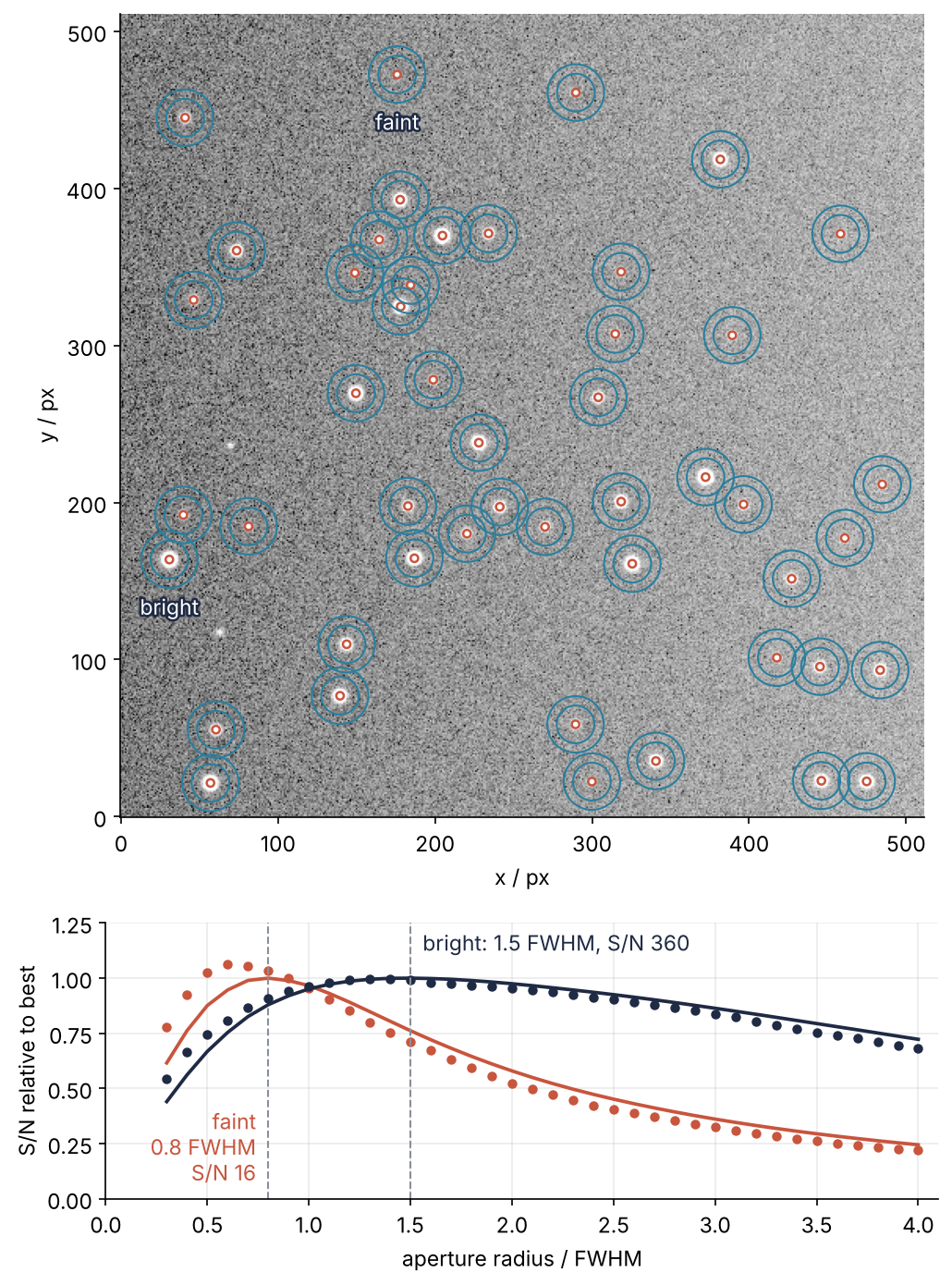
This is where we end up. On top, the frame with the chosen circle and sky ring on every star; below, the signal-to-noise of two stars against radius, dots measured on 400 noisy copies of each star, lines predicted from the one frame by the CCD equation and its curve of growth. The faint star, 1,654 e⁻, does best at 0.8 FWHM and loses fast beyond it. The brightest, 150,000 e⁻, peaks at 1.5 FWHM on a curve so flat that anything from 1 to 2 FWHM stays within 5 % of the best. The rule of thumb "radius equals the FWHM" is right for neither, though it costs each under 5 %.

Setup

The frame is in electrons: a real frame in ADU, the counts the camera writes, is multiplied by the gain from its header first. The cell places the stars at random and adds sky, Poisson noise, and read noise; you need not study it, and the seeded generator is the subject of Random numbers with numpy.random. One thing in it matters later. Each star is a Moffat profile, a bell like a Gaussian with wider wings, which is the shape seeing gives, and enclosed_fraction(r) is the fraction of a star's light inside radius \(r\) for that profile, in closed form.

import numpy as np
import matplotlib.pyplot as plt
import matplotlib.patheffects as pe
from astropy.stats import sigma_clipped_stats, SigmaClip
from astropy.visualization import ImageNormalize, ZScaleInterval, AsinhStretch
from photutils.detection import DAOStarFinder
from photutils.aperture import (CircularAperture, CircularAnnulus,
                                aperture_photometry, ApertureStats)
from photutils.utils import calc_total_error

N = 512                               # frame size, px
FWHM = 3.0                            # seeing, px: 1.2 arcsec at 0.4 arcsec per pixel
BETA = 4.765                          # Moffat exponent that matches atmospheric turbulence
SKY_LEFT, SKY_RIGHT = 200.0, 230.0    # sky, e⁻ per pixel, rising from left to right
READ_NOISE = 5.0                      # e⁻ per pixel
T_EXP = 60.0                          # exposure, s
rng = np.random.default_rng(146)


def moffat_alpha(fwhm):
    return fwhm / (2 * np.sqrt(2 ** (1 / BETA) - 1))


def enclosed_fraction(r, fwhm=FWHM):
    """Fraction of a star's light inside radius r (px)."""
    return 1 - (1 + r**2 / moffat_alpha(fwhm)**2) ** (1 - BETA)


def moffat_stamp(dx, dy, flux, fwhm=FWHM, size=41, sub=5):
    """A star of `flux` e⁻ on a size × size stamp, offset dx, dy px from its central pixel."""
    s = (np.arange(size * sub) + 0.5) / sub - size / 2       # sub-pixel centers
    x, y = np.meshgrid(s - dx, s - dy)
    fine = (1 + (x**2 + y**2) / moffat_alpha(fwhm)**2) ** (-BETA)
    stamp = fine.reshape(size, sub, size, sub).sum(axis=(1, 3))
    return flux * stamp / stamp.sum()


def free(p, others):
    return all(np.hypot(*(p - o)) >= 25 for o in others)


xy = []
while len(xy) < 48:
    p = rng.uniform(21, N - 22, 2)
    if free(p, xy):
        xy.append(p)
while True:                           # a faint star 15 px from a bright one, for the second pitfall
    bright_xy = rng.uniform(21, N - 22, 2)
    angle = rng.uniform(0, 2 * np.pi)
    faint_xy = bright_xy + 15 * np.array([np.cos(angle), np.sin(angle)])
    if free(bright_xy, xy) and free(faint_xy, xy) and np.all((faint_xy >= 21) & (faint_xy <= N - 22)):
        xy += [bright_xy, faint_xy]
        break
true_xy = np.array(xy)
true_flux = np.concatenate([rng.permutation(np.geomspace(1500, 150_000, 48)), [80_000, 2_000]])

noiseless = np.tile(SKY_LEFT + (SKY_RIGHT - SKY_LEFT) * np.arange(N) / (N - 1), (N, 1))
for (x, y), F in zip(true_xy, true_flux):
    ix, iy = int(round(x)), int(round(y))
    noiseless[iy - 20:iy + 21, ix - 20:ix + 21] += moffat_stamp(x - ix, y - iy, F)
frame = rng.poisson(noiseless) + rng.normal(0, READ_NOISE, (N, N))

plt.rcParams.update({
    "figure.figsize": (7, 3.6), "figure.dpi": 110,
    "axes.spines.top": False, "axes.spines.right": False,
    "axes.grid": True, "grid.alpha": 0.25,
    "font.size": 11, "lines.linewidth": 1.8,
})
INK, ACCENT, SECOND, MUTED = "#1f2a44", "#c8553d", "#2a7f9e", "#8a8f98"

print(f"{N} × {N} px, {len(true_flux)} stars from {true_flux.min():,.0f} to {true_flux.max():,.0f} e⁻, "
      f"FWHM {FWHM} px, noise in empty sky {np.sqrt(215 + READ_NOISE**2):.1f} e⁻ per pixel")

512 × 512 px, 50 stars from 1,500 to 150,000 e⁻, FWHM 3.0 px, noise in empty sky 15.5 e⁻ per pixel

Step 1: Measure the sky and its noise with sigma_clipped_stats

On a linear gray scale the frame is black with a few white dots, since the brightest star peaks 50 times above the sky. An asinh stretch compresses the bright end, and the zscale interval sets the display limits near the sky level, from a sample of pixels:

Copy

norm = ImageNormalize(frame, interval=ZScaleInterval(), stretch=AsinhStretch())
fig, ax = plt.subplots(figsize=(6.5, 6.5))
ax.imshow(frame, cmap="gray", norm=norm, origin="lower")
ax.set(xlabel="x / px", ylabel="y / px")
ax.grid(False)
plt.show()

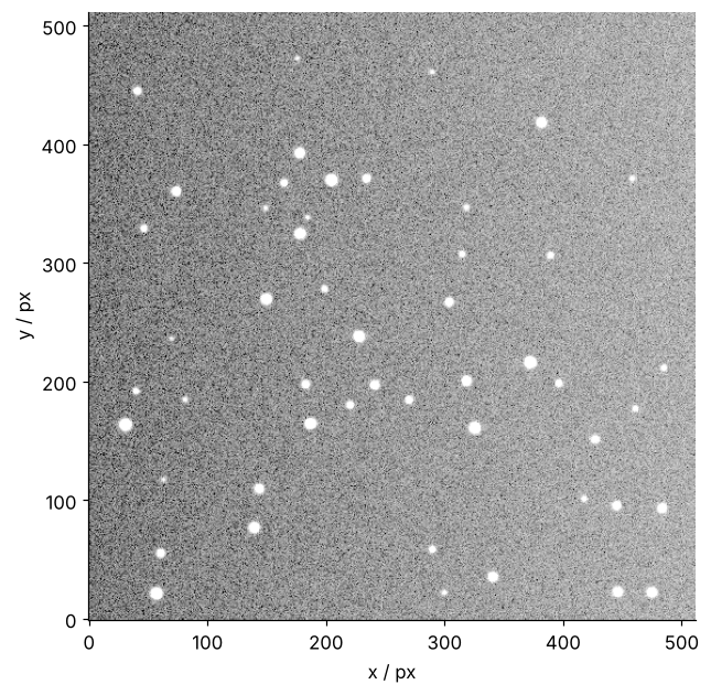
The sky level is the typical pixel value, and the stars get in the way. Sigma clipping removes them: drop every pixel more than 3 standard deviations from the median, recompute median and standard deviation from what is left, and repeat (up to five times by default). Star pixels are the outliers it drops.

print(f"all pixels: mean {frame.mean():6.1f}  median {np.median(frame):6.1f}  std {frame.std():6.1f} e⁻")
mean, median, std = sigma_clipped_stats(frame, sigma=3.0)
print(f"clipped:    mean {mean:6.1f}  median {median:6.1f}  std {std:6.1f} e⁻")
noise, ramp = np.sqrt(215 + READ_NOISE**2), (SKY_RIGHT - SKY_LEFT) / np.sqrt(12)
print(f"noise {noise:.1f} e⁻ and ramp {ramp:.1f} e⁻ in quadrature: {np.hypot(noise, ramp):.1f} e⁻")

all pixels: mean  221.4  median  215.2  std  134.6 e⁻
clipped:    mean  215.2  median  214.9  std   17.6 e⁻
noise 15.5 e⁻ and ramp 8.7 e⁻ in quadrature: 17.7 e⁻

The stars pull the plain standard deviation up to 134.6 e⁻. The clipped 17.6 e⁻ is more than the 15.5 e⁻ of pure noise, because the sky's 30 e⁻ rise across the frame spreads the values by another 8.7 e⁻, the standard deviation of values spread evenly over 30 e⁻ (30/√12), and in quadrature that is 17.7 e⁻. The frame is what Setup says, and one sky value for the whole frame is already not quite right.

Step 2: Find the stars with DAOStarFinder

DAOStarFinder smooths the image with a Gaussian of the given FWHM and keeps the peaks above a threshold that are round and sharp enough to be stars: the threshold and the objects of Counting cells with scipy.ndimage, plus a test of shape. The threshold is five times the sky noise, on the frame minus the sky:

finder = DAOStarFinder(threshold=5 * std, fwhm=FWHM)
sources = finder(frame - median)
table = sources["x_centroid", "y_centroid", "peak", "flux"][:5]
for col in table.colnames:
    table[col].info.format = ".1f"
print(table)

x_centroid y_centroid  peak    flux 
---------- ---------- ------ -------
      57.0       21.4 9135.9 71280.1
     299.9       22.3  202.3  1682.7
     446.1       22.8 3426.9 24981.9
     474.9       22.4 4126.6 32566.2
     340.7       35.4 3328.0 26184.3

The result is an astropy Table, one row per star, with columns picked by name and the centroid in pixels. The flux column is the sum of the frame's values inside the finder's kernel footprint, with no local sky taken off, so it is not a measurement you can use.

Match each detection to the nearest true star and see what was missed:

found_xy = np.column_stack([sources["x_centroid"], sources["y_centroid"]])
dist = np.linalg.norm(found_xy[:, None] - true_xy[None], axis=2)    # detections × true stars, px
idx = dist.argmin(axis=1)
print(f"found {len(sources)} of {len(true_flux)}, largest position error {dist.min(axis=1).max():.2f} px")
for k in sorted(set(range(len(true_flux))) - set(idx)):
    sky_there = SKY_LEFT + (SKY_RIGHT - SKY_LEFT) * true_xy[k, 0] / (N - 1)
    print(f"missed: x = {true_xy[k, 0]:5.1f} px, {true_flux[k]:,.0f} e⁻, sky {sky_there - median:+.1f} e⁻ against the median")

order = np.argsort(idx)                                     # true order, for the checks below
positions, F_true = found_xy[order], true_flux[idx[order]]
planted = np.flatnonzero(idx[order] >= 48)                  # the pair placed for the pitfall

found 48 of 50, largest position error 0.13 px
missed: x =  69.8 px, 1,500 e⁻, sky -10.8 e⁻ against the median
missed: x =  63.1 px, 1,825 e⁻, sky -11.2 e⁻ against the median

Forty-eight of 50, each centroid within 0.13 px of the truth. The missed stars are the faintest and the third faintest; the second faintest, 1,654 e⁻, was found and becomes the faint star of Step 3. Both missed sit near the left edge, where the true sky is 11 e⁻ per pixel below the median that was subtracted. Steps 3 to 6 work with the 48: positions holds their detected centroids, and F_true their true fluxes, used only to check the results.

Step 3: Put apertures and annuli on the stars and subtract the local sky

A CircularAperture of radius 3 px, one FWHM, holds the star. A CircularAnnulus, a ring from 12 to 18 px, holds the sky around it. The ring sits that far out because almost no starlight reaches it: enclosed_fraction(12) is 0.99988. The sky per pixel is the sigma-clipped median of the ring, which follows the gradient that one global value missed:

aperture = CircularAperture(positions, r=3.0)
annulus = CircularAnnulus(positions, r_in=12.0, r_out=18.0)
sky_stats = ApertureStats(frame, annulus, sigma_clip=SigmaClip(sigma=3.0))
sky, sky_std = sky_stats.median, sky_stats.std        # e⁻ per pixel, one value per star
n_pix, n_sky = aperture.area, annulus.area
sky_noise = np.median(sky_std)
print(f"enclosed fraction at 12 px {enclosed_fraction(12.0):.5f}, sky noise in the rings {sky_noise:.1f} e⁻")

enclosed fraction at 12 px 0.99988, sky noise in the rings 15.3 e⁻

Across a ring 36 px wide the sky rises by about 2 e⁻, so the ring's noise, 15.3 e⁻, is the pure noise that Step 1 could not separate from the ramp.

aperture.area is the circle's area, 28.3 px² for 3 px, not a count of pixels. photutils weights a pixel on the rim by the fraction of it inside the circle, so a pixel half inside adds half its value.

The error of the sum has two parts. The first is the noise of the pixels inside the circle. Photon counts are Poisson distributed, with a variance equal to the count, and the variances of independent noises add. calc_total_error builds a per-pixel error from the sky noise and the Poisson noise of the stars. It wants the frame minus the sky: hand it the raw frame and the sky's Poisson noise is counted twice, once in the frame and once in the sky noise. Step 1's global median will do, since the 15 e⁻ by which it misses the sky at the edges change a pixel's variance of 234 e⁻² by at most 15 e⁻², and effective_gain=1.0 because the frame is already in electrons. The second part is the sky estimate itself, a clipped median over \(n_\text{sky}\) noisy ring pixels and so uncertain by about \(\sigma_\text{sky}/\sqrt{n_\text{sky}}\) per pixel (the standard error of the mean; a median's is a quarter larger, too little to matter here). The same estimate is subtracted from all \(n_\text{pix}\) pixels in the circle, so its error is multiplied by \(n_\text{pix}\), not added \(n_\text{pix}\) times in quadrature. A larger ring shrinks it.

error = calc_total_error(frame - median, np.full(frame.shape, sky_noise), effective_gain=1.0)
phot = aperture_photometry(frame, aperture, error=error)
total = np.asarray(phot["aperture_sum"])
net = total - sky * n_pix
net_err = np.hypot(phot["aperture_sum_err"], n_pix * sky_std / np.sqrt(n_sky))

by_flux = np.argsort(F_true)
print(" true F      sum      sky     net   error  / e⁻")
for k in by_flux[[0, 12, 24, 36, -1]]:
    print(f"{F_true[k]:7,.0f} {total[k]:8,.0f} {sky[k] * n_pix:8,.0f} {net[k]:7,.0f} {net_err[k]:7,.0f}")

 true F      sum      sky     net   error  / e⁻
  1,654    7,326    5,938   1,388      87
  5,361   10,465    5,988   4,477     102
 17,375   20,548    6,024  14,524     142
 56,307   52,945    6,442  46,503     227
150,000  129,614    5,673 123,941     354

For the faintest row the sky in the circle, 5,938 e⁻, is four times the star's 1,388 e⁻. Every faint star here is mostly sky.

Step 4: Turn fluxes into magnitudes and measure the curve of growth

The magnitude follows from the net flux, and its error from the derivative of the logarithm, \(\sigma_m = (2.5/\ln 10)\,\sigma_F/F = 1.0857\,\sigma_F/F\):

m = -2.5 * np.log10(net / T_EXP)
m_err = 2.5 / np.log(10) * net_err / net
m_true = -2.5 * np.log10(F_true / T_EXP)
print(f"measured minus true: median {np.median(m - m_true):+.3f} mag")

measured minus true: median +0.208 mag

The stars come out 0.208 mag too faint in the median, because the circle misses the light outside 3 px. How much it misses can be read off the frame. The curve of growth is a star's sky-subtracted flux inside a growing radius, divided by its flux at a radius large enough to hold all of it, here 4 FWHM. Take the ten brightest stars with no neighbor inside 18 px, the outer edge of the ring: bright because their curves are the least noisy, alone because a neighbor's light would bend the curve. aperture_photometry takes a list of apertures and returns one numbered column per radius, aperture_sum_0, aperture_sum_1, and so on. (photutils.profiles.CurveOfGrowth does the same for one star at a time.)

gaps = np.linalg.norm(positions[:, None] - positions[None], axis=2)
np.fill_diagonal(gaps, np.inf)
isolated = gaps.min(axis=1) > 18
cog_stars = [k for k in np.argsort(net)[::-1] if isolated[k]][:10]

radii = FWHM * np.arange(0.3, 4.01, 0.1)                    # px
apertures = [CircularAperture(positions[cog_stars], r=r) for r in radii]
cog = aperture_photometry(frame, apertures)
growth = np.array([cog[f"aperture_sum_{i}"] - sky[cog_stars] * a.area for i, a in enumerate(apertures)])
ee = np.median(growth / growth[-1], axis=1)                 # enclosed fraction, median of ten stars

for f in [0.5, 1.0, 1.5, 2.0]:
    i = np.argmin(abs(radii - f * FWHM))
    closed = enclosed_fraction(radii[i]) / enclosed_fraction(radii[-1])
    print(f"r = {f:.1f} FWHM: measured {ee[i]:.3f}, closed form {closed:.3f}")
i_fwhm = np.argmin(abs(radii - FWHM))
offset = -2.5 * np.log10(ee[i_fwhm])
print(f"offset at 1 FWHM: {offset:+.3f} mag")

r = 0.5 FWHM: measured 0.395, closed form 0.422
r = 1.0 FWHM: measured 0.823, closed form 0.840
r = 1.5 FWHM: measured 0.958, closed form 0.964
r = 2.0 FWHM: measured 0.988, closed form 0.991
offset at 1 FWHM: +0.212 mag

The measured curve runs a little below the closed form, 0.823 against 0.840 at 1 FWHM. A pixel records the average of the profile over its square, which widens the spot, and the closed form knows nothing of pixels. The frame's own curve predicts an offset of +0.212 mag, the closed form +0.190, and the stars show +0.208. Use the curve from the frame.

Copy

fig, ax = plt.subplots(figsize=(7, 3.4))
ax.errorbar(m_true, m - m_true, yerr=m_err, fmt="o", ms=4, capsize=2, lw=1, color=INK)
ax.axhline(offset, color=SECOND, ls="--", lw=1)
ax.text(m_true.min(), offset + 0.04, f"curve of growth: {offset:+.2f} mag", color=SECOND)
ax.set(xlabel="true m / mag", ylabel="Δm / mag")
plt.show()

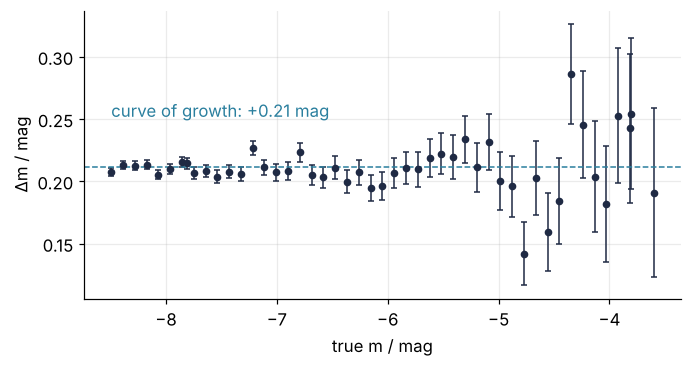
The bright stars on the left sit on the line; the faint ones on the right scatter around it by their error bars.