Random forests with scikit-learn: which variables decide the yield?

The problem: six process variables, one yield

Here is the log of 500 runs of a chemical reactor. Each run records six process variables, temperature, pressure, residence time, catalyst load, stirring speed, and feed purity, and the yield in %, which scatters by 3 points between runs at the same settings. The question is the one every process engineer asks of such a table: which of the six move the yield, and how? A fermenter log with temperature, pH, feed rate, and inoculum poses the same question.

A random forest answers it well, and its most convenient answer is wrong. The importance a fitted forest reports out of the box credits a variable with many distinct values even when it does nothing. A linear fit fails the other way: it misses a variable that acts only together with another. The data here are simulated from a known formula, given in Setup, so every ranking can be checked against the truth.

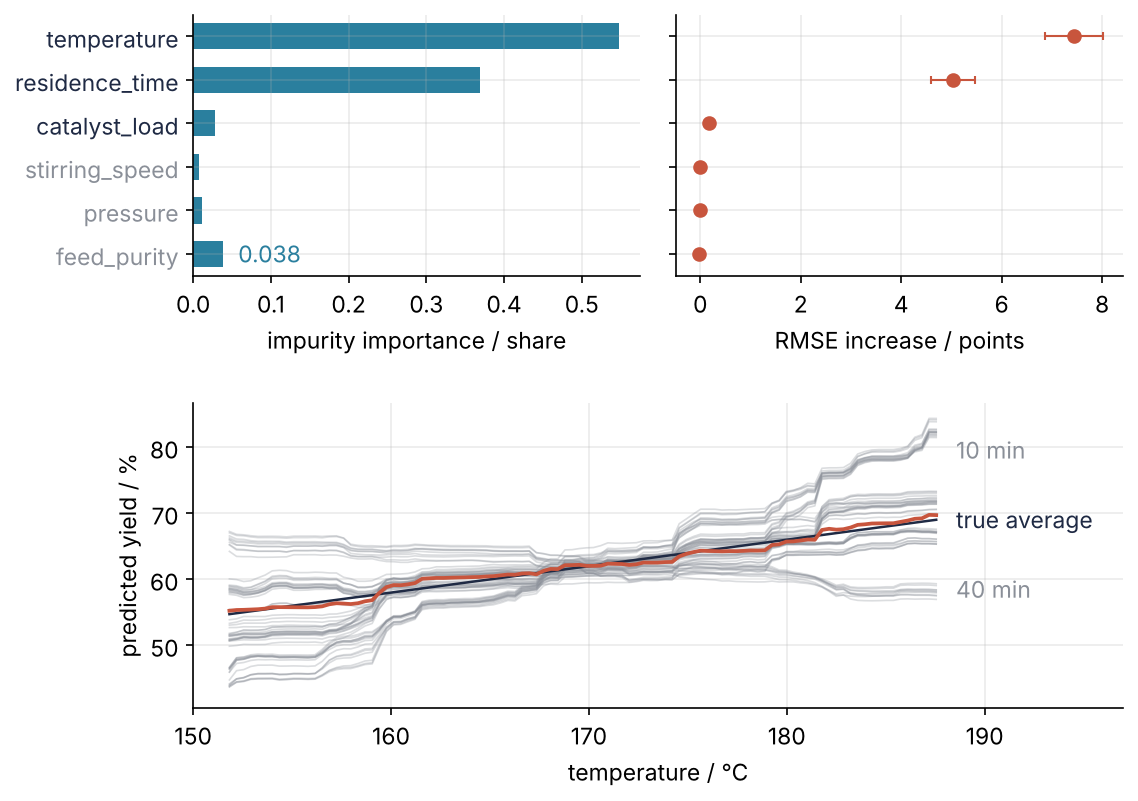
This is where we end up. The top row ranks the six variables twice, by the importance the forest computes on its own training data and by how much its error on unseen runs grows when a variable is scrambled; the bottom panel shows what the forest learned about temperature. The split, cross-validation, and decision trees come from Classification with scikit-learn.

Setup

The yield in % follows this formula, with \(t\), \(s\), and \(c\) the temperature, residence time, and catalyst load scaled linearly from their logged ranges onto \(-1\) to \(1\), and \(\varepsilon\) the run-to-run scatter, normal with a standard deviation of 3 points:

Temperature acts strongly, residence time only through its product with temperature, catalyst load a little, and pressure, stirring speed, and feed purity not at all.

import numpy as np
import pandas as pd
import matplotlib.pyplot as plt
from sklearn.ensemble import RandomForestRegressor
from sklearn.linear_model import LinearRegression
from sklearn.model_selection import train_test_split, GridSearchCV
from sklearn.inspection import permutation_importance, PartialDependenceDisplay
from sklearn.metrics import root_mean_squared_error

plt.rcParams.update({
    "figure.figsize": (7, 3.6), "figure.dpi": 110,
    "axes.spines.top": False, "axes.spines.right": False,
    "axes.grid": True, "grid.alpha": 0.25,
    "font.size": 11, "lines.linewidth": 1.8,
})
INK, ACCENT, SECOND, MUTED = "#1f2a44", "#c8553d", "#2a7f9e", "#8a8f98"

SEED = 2
rng = np.random.default_rng(SEED)
n = 500
runs = pd.DataFrame({
    "temperature": np.round(rng.uniform(150, 190, n), 1),         # °C, measured
    "pressure": rng.choice([2, 3, 4, 5], n),                        # bar, setpoint
    "residence_time": rng.choice([10, 20, 30, 40], n),              # min, setpoint
    "catalyst_load": rng.choice([0.5, 1.0, 1.5, 2.0], n),           # mol %, charge
    "stirring_speed": rng.choice([300, 450, 600], n),               # rpm, setpoint
    "feed_purity": np.round(rng.uniform(97.0, 99.9, n), 2),         # %, lab assay
})

def true_mean(df):
    """The formula without the scatter: the yield a perfect model would predict."""
    t = (df["temperature"] - 170) / 20
    s = (df["residence_time"] - 25) / 15
    c = (df["catalyst_load"] - 1.25) / 0.75
    return (62 + 8 * t - 12 * t * s + 1.5 * c).to_numpy()

yield_pct = true_mean(runs) + rng.normal(0, 3, n)   # "yield" is a Python keyword
print(runs.shape)

(500, 6)

Step 1: Split the runs and fit a linear baseline

A quarter of the runs go into a test set, as in the prerequisite, and scikit-learn keeps the DataFrame's column names. The error measure throughout is the root-mean-square error (RMSE), the typical size of a prediction's miss, in points of yield. The cell then ranks the variables by the linear fit. A coefficient is a slope per °C or per rpm, so its size depends on the unit; multiplied by the logged range of its variable, it becomes the change in yield across the log, in points, and the six can be compared:

X_train, X_test, y_train, y_test = train_test_split(runs, yield_pct, test_size=0.25, random_state=0)

linear = LinearRegression().fit(X_train, y_train)
rmse_linear = root_mean_squared_error(y_test, linear.predict(X_test))
rmse_floor = root_mean_squared_error(y_test, true_mean(X_test))
print(f"test RMSE: linear {rmse_linear:.2f} points, the formula itself {rmse_floor:.2f} points")

effect = pd.Series(linear.coef_, index=runs.columns) * (runs.max() - runs.min())
for name, value in effect.sort_values(key=abs, ascending=False).items():
    print(f"{name:15s} {value:+5.1f} points over the logged range")

test RMSE: linear 6.18 points, the formula itself 2.77 points
temperature     +16.5 points over the logged range
catalyst_load    +4.2 points over the logged range
stirring_speed   +1.4 points over the logged range
feed_purity      +1.1 points over the logged range
residence_time   +0.4 points over the logged range
pressure         +0.3 points over the logged range

The linear fit misses by 6.18 points. The formula itself misses these 125 runs by 2.77, their scatter, which no model can beat; on real data the scatter of repeated runs at the same settings stands in for it. Temperature and catalyst load are found. Residence time ranks fifth, below stirring speed and feed purity, which the formula leaves out.

Show code

Copy

fig, ax = plt.subplots()
for minutes, fill in [(10, MUTED), (40, "none")]:    # runs in gray, as in Step 6; filled or open
    pick = runs["residence_time"] == minutes
    ax.plot(runs.loc[pick, "temperature"], yield_pct[pick], "o", ms=4, color=MUTED, mfc=fill, mew=1)
    end = runs.loc[pick, "temperature"].idxmax()
    ax.text(191, true_mean(runs.loc[[end]])[0], f"{minutes} min", color=MUTED, va="center")
ax.set(xlabel="temperature / °C", ylabel="yield / %", xlim=(148, 198))
plt.show()

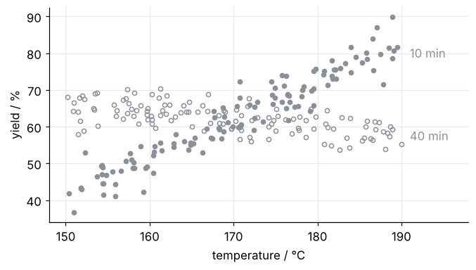
Averaged over the four residence times, the temperature slope is positive and residence time does nothing, and that average is all a linear model can hold. The real slope rises steeply at 10 min and turns slightly negative at 40 min. A plane has one slope per variable.

Step 2: Grow a random forest and read its out-of-bag error

A regression tree asks the same yes-or-no questions as the classification tree of the prerequisite, but a leaf predicts the mean yield of the training runs that end in it, and each question is chosen to make the yields on either side as alike as possible. A deep tree fits the noise.

The fix is to grow many trees, each on its own bootstrap sample of the training runs: as many runs as there are, drawn with replacement, so that about 63 % of the distinct runs make it in (bootstrap confidence intervals use the same resampling). The trees then differ, and the forest predicts their average, in which much of their scatter cancels. Breiman's original forest also lets each split look at only a random subset of the variables; scikit-learn's regressor by default lets every split consider all six, so the bootstrap is the only difference between its trees. The knobs are n_estimators, the number of trees, and max_depth and min_samples_leaf, which limit how far each tree grows. max_features returns in Variations.

Each run is left out of about 37 % of the bootstrap samples. Averaged over only those trees, its prediction comes from trees that never saw it: the out-of-bag prediction, a held-out error without held-out data. oob_score=True stores it in oob_prediction_, the middle row below:

forest = RandomForestRegressor(oob_score=True, random_state=0).fit(X_train, y_train)
for label, y_true, y_pred in [("training", y_train, forest.predict(X_train)),
                              ("out-of-bag", y_train, forest.oob_prediction_),
                              ("test", y_test, forest.predict(X_test))]:
    print(f"{label:10s} RMSE {root_mean_squared_error(y_true, y_pred):.2f} points")

training   RMSE 1.26 points
out-of-bag RMSE 3.46 points
test       RMSE 3.47 points

The training error of 1.26 points lies far below the 2.77-point floor, so it measures memory, not skill (Overfitting shows why). The out-of-bag error, 3.46, agrees with the test error, 3.47. The attribute oob_score_ holds the same prediction's R², not an error in points.

for n_trees in [25, 50, 100, 200, 500]:
    f = RandomForestRegressor(n_estimators=n_trees, oob_score=True, random_state=0).fit(X_train, y_train)
    print(f"{n_trees:4d} trees   out-of-bag RMSE {root_mean_squared_error(y_train, f.oob_prediction_):.2f} points")

  25 trees   out-of-bag RMSE 3.57 points
  50 trees   out-of-bag RMSE 3.51 points
 100 trees   out-of-bag RMSE 3.46 points
 200 trees   out-of-bag RMSE 3.44 points
 500 trees   out-of-bag RMSE 3.42 points

More trees never hurt. Past 100 they barely help: 3.46 points becomes 3.42 at 500.

Step 3: Tune depth and number of trees with GridSearchCV

GridSearchCV runs the prerequisite's cross-validation loop for every combination in a grid and then refits the best one on the whole training set. scikit-learn always maximizes a score, so an error enters with a minus sign:

grid = GridSearchCV(RandomForestRegressor(random_state=0),
                    {"max_depth": [2, 4, 6, 8, None], "n_estimators": [50, 200, 500]},
                    cv=5, scoring="neg_root_mean_squared_error").fit(X_train, y_train)

cv = pd.DataFrame(grid.cv_results_)
cv["max_depth"] = cv["param_max_depth"].astype(object).fillna("none").astype(str)
table = cv.pivot(index="max_depth", columns="param_n_estimators", values="mean_test_score")
print("cross-validated RMSE / points, rows max_depth, columns n_estimators")
print((-table).round(2).to_string())
print(f"fold spread {cv['std_test_score'].min():.2f} to {cv['std_test_score'].max():.2f} points")
print("best:", grid.best_params_)

best = grid.best_estimator_
rmse_tuned = root_mean_squared_error(y_test, best.predict(X_test))
closed = (rmse_linear - rmse_tuned) / (rmse_linear - rmse_floor)
print(f"test RMSE: tuned forest {rmse_tuned:.2f} points, {closed * 100:.0f} % of the way from linear to the formula")

cross-validated RMSE / points, rows max_depth, columns n_estimators
param_n_estimators   50    200   500
max_depth                           
2                   4.85  4.86  4.86
4                   3.67  3.63  3.61
6                   3.54  3.49  3.48
8                   3.57  3.50  3.49
none                3.57  3.50  3.49
fold spread 0.22 to 0.45 points
best: {'max_depth': 6, 'n_estimators': 500}
test RMSE: tuned forest 3.28 points, 85 % of the way from linear to the formula

Depth 2 misses by 4.86 points and depth 4 by about 3.6, while depth 6, 8, and unlimited tie at 3.5, well inside the fold spread of 0.22 to 0.45 points. The number of trees moves only the second decimal, as Step 2's loop already showed. The search picks depth 6 with 500 trees, and on the test set the tuned forest misses by 3.28 points, against 6.18 for the linear fit and 2.77 for the formula: it closes 85 % of the gap. Of the two knobs, only the depth is worth a search.

Step 4: Read the forest's built-in importance

The impurity of a node in a regression tree is the mean squared deviation of its training yields from their mean. Every split lowers it: the two halves, weighted by their numbers of runs, have less impurity together than the node they came from, and the decrease is credited to the variable the split asks about. feature_importances_ adds up these decreases per variable over each tree, scales each tree's sums to 1, and averages them over the trees. It is the mean decrease in impurity:

impurity = pd.Series(best.feature_importances_, index=runs.columns).sort_values(ascending=False)
for name, value in impurity.items():
    print(f"{name:15s} {value:.3f}")
print(f"feed purity in the {len(X_train)} training runs: {X_train['feed_purity'].nunique()} distinct values")

temperature     0.548
residence_time  0.368
feed_purity     0.038
catalyst_load   0.028
pressure        0.011
stirring_speed  0.007
feed purity in the 375 training runs: 212 distinct values

Temperature and residence time lead, as the formula says. Then feed purity, which the formula does not contain, ranks third, above catalyst load, which it does, and at more than three times pressure and five times stirring speed, the two other variables that do nothing. The cause is the last line: feed purity takes 212 distinct values in the 375 training runs, 211 places to split, against two or three for a setpoint column, and with that many chances a tree of depth 6 finds splits on feed purity that lower the training error by fitting noise. The importance counts them as real, because it is computed on the training data. This is the known bias of impurity importance toward variables with many distinct values.