Overfitting: why the model that fits its data best predicts worst (Python)

The question

A logger on the wall of a lab reads the room temperature every 72 minutes: 20 readings over one day, from 0:00 to 22:48, each scattered by the logger's 0.2 K. At 14:30 you took a measurement that depends on the room temperature, and 14:30 is not one of the readings. The everyday answer is a smooth curve through the readings, and the simplest smooth curve is a polynomial, whose degree you choose. Choose it badly and the curve overfits: it follows the readings closely and the room poorly.

Show code

import numpy as np
import matplotlib.pyplot as plt
from numpy.polynomial import Polynomial

plt.rcParams.update({
    "figure.figsize": (7, 3.6), "figure.dpi": 110,
    "axes.spines.top": False, "axes.spines.right": False,
    "axes.grid": True, "grid.alpha": 0.25,
    "font.size": 11, "lines.linewidth": 1.8,
})
INK, ACCENT, SECOND, MUTED = "#1f2a44", "#c8553d", "#2a7f9e", "#8a8f98"

# The readings are simulated from a known curve, so that every answer can be checked.
def truth(t):
    """Room temperature in °C at t hours: night setback, heating on near 7:00, setback near 18:00."""
    return 19.5 + 2.5 / (1 + np.exp(-(t - 7) / 1.5)) - 2.0 / (1 + np.exp(-(t - 18) / 1.5))

SIGMA = 0.2                                        # K, the logger's scatter
N, T_END = 20, 22.8                                # readings, hours
t_train = np.linspace(0, T_END, N)                 # one reading every 72 min
rng = np.random.default_rng(247)
y_train = truth(t_train) + SIGMA * rng.standard_normal(N)
t_test = np.sort(rng.uniform(0, T_END, N))         # fresh readings, inside the same span, never fitted
y_test = truth(t_test) + SIGMA * rng.standard_normal(N)
print(f"{N} readings from {t_train[0]:.1f} h to {t_train[-1]:.1f} h, "
      f"every {60 * (t_train[1] - t_train[0]):.0f} min, scatter {SIGMA} K")

fig, ax = plt.subplots()
ax.plot(t_train, y_train, "o", ms=6, color=INK)
ax.set(xlabel="time of day / h", ylabel="temperature / °C", xlim=(0, 24), xticks=[0, 6, 12, 18, 24])
plt.show()

20 readings from 0.0 h to 22.8 h, every 72 min, scatter 0.2 K

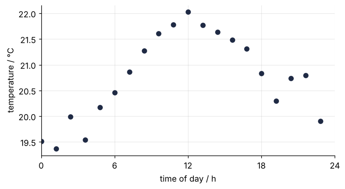
Twenty temperature readings in °C against time of day in hours, one every 72 minutes. Low and flat at night, a rise in the morning, a plateau through the day, a drop in the evening, with a jitter of about 0.2 K.

Two things are obvious. The room is cool at night, warms in the morning when the heating comes on, and cools again in the evening. Around whatever the room is doing, the readings jitter by about 0.2 K, the logger's scatter.

What is missing is a formula. When physics gives you the form of a curve, an exponential decay or a Michaelis-Menten rate, fit that form and its few parameters, as in curve_fit from the ground up. A day of heating, setback, open doors, and afternoon sun has no such form, and that is when people reach for a polynomial or a spline.

The plan a scientist would make is a least-squares fit of a polynomial. Every extra degree lets the curve pass closer to the readings, so a high degree looks like the safe choice.

Less obvious: is the curve that fits the 20 readings best also the one that gives the best temperature at 14:30? And if it is not, how do you choose the degree without knowing the true curve? The readings are simulated from a known curve, so every answer here can be checked against it. I picked seed 247 because its single draw shows what the average over a thousand draws shows.

The idea: a flexible curve fits the noise too

A polynomial of degree d has d + 1 coefficients and can bend up to d − 1 times. The first few bends go to the shape of the day, the morning ramp and the evening drop. Once those are followed, there is nothing left to follow but the logger's scatter, and every further bend chases a reading that happens to sit high or low. Chasing the scatter costs nothing at the readings the fit sees. Between them it costs everything, because the next reading's scatter has nothing to do with the last one's.

To see it, I drew 20 fresh readings at random times of the same day, from the same curve with the same scatter, and never show them to the fit. The training error is the root-mean-square (RMS) misfit to the 20 readings the fit used; the test error is the same on the 20 fresh ones. Here are three degrees:

Show code

def rms(residuals):
    return np.sqrt(np.mean(residuals ** 2))

t_fine = np.linspace(0, T_END, 1000)
YLIM = (18.6, 23.0)
fig, axes = plt.subplots(3, 1, figsize=(7, 6.6), sharex=True, sharey=True)
for ax, d in zip(axes, [1, 3, 15]):
    p = Polynomial.fit(t_train, y_train, d)
    curve = p(t_fine)
    ax.plot(t_fine, truth(t_fine), color=MUTED, lw=1, ls="--", label="the curve the readings were drawn from")
    ax.plot(t_fine, np.clip(curve, YLIM[0] - 1, YLIM[1] + 1), color=ACCENT, label="the fit")
    ax.plot(t_train, y_train, "o", ms=5, color=INK, label="readings, fitted")
    ax.plot(t_test, y_test, "o", ms=5, mfc="white", mec=SECOND, mew=1.2, label="fresh readings, never fitted")
    ax.text(0.01, 0.96, f"degree {d}    training {rms(y_train - p(t_train)):.2f} K · fresh {rms(y_test - p(t_test)):.2f} K",
            transform=ax.transAxes, va="top")
    if curve.min() < YLIM[0]:
        i = np.argmin(curve)
        j = i + np.argmax(curve[i:] >= YLIM[0])             # where the dive comes back into view
        ax.annotate(f"down to {curve[i]:.1f} °C", xy=(t_fine[j], YLIM[0] + 0.05), xytext=(t_fine[j] + 1.2, YLIM[0] + 0.12),
                    color=ACCENT, va="bottom", arrowprops=dict(arrowstyle="->", color=ACCENT, lw=1, shrinkA=0, shrinkB=2))
fig.legend(*axes[0].get_legend_handles_labels(), frameon=False, loc="lower center", bbox_to_anchor=(0.5, 0.88), ncol=2)
axes[1].set_ylabel("temperature / °C")
axes[-1].set(xlabel="time of day / h", xlim=(0, 24), xticks=[0, 6, 12, 18, 24], ylim=YLIM)
plt.show()

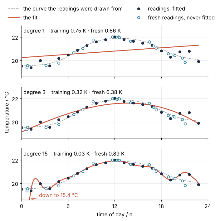
Temperature in °C against time of day, fits of degree 1, 3, and 15 through 20 filled readings, with hollow fresh readings and the dashed true curve. Degree 1 misses the ramps, degree 3 rounds them off, degree 15 threads every filled reading and dives off the axis near midnight.

Degree 1 is a straight line through a day with two ramps. It misses both sets by about the same amount, 0.75 K and 0.86 K, and is said to underfit. Degree 3 follows the day but rounds off its corners, 0.32 K and 0.38 K. Degree 15 threads the readings to 0.03 K and dives to 15.4 °C between the first two of them, so the two fresh readings in the first hour are missed by kelvins. Its test error, 0.89 K, is worse than the straight line's.

The training error carries one warning on its own. No curve knows the logger's scatter in advance, so a fit that comes within 0.03 K of the readings, about a sixth of the 0.2 K the logger scatters by, has followed that scatter. The converse does not hold. Every fit absorbs a little of the scatter, so an honest fit lands somewhat below 0.2 K: degree 4 reaches 0.22 K in this draw and degree 6 0.18 K, and the formalization says how far below to expect. The training error cannot tell you where to stop. That is what the fresh readings are for. Watch the degree climb from 1 to 15 with both errors traced out below:

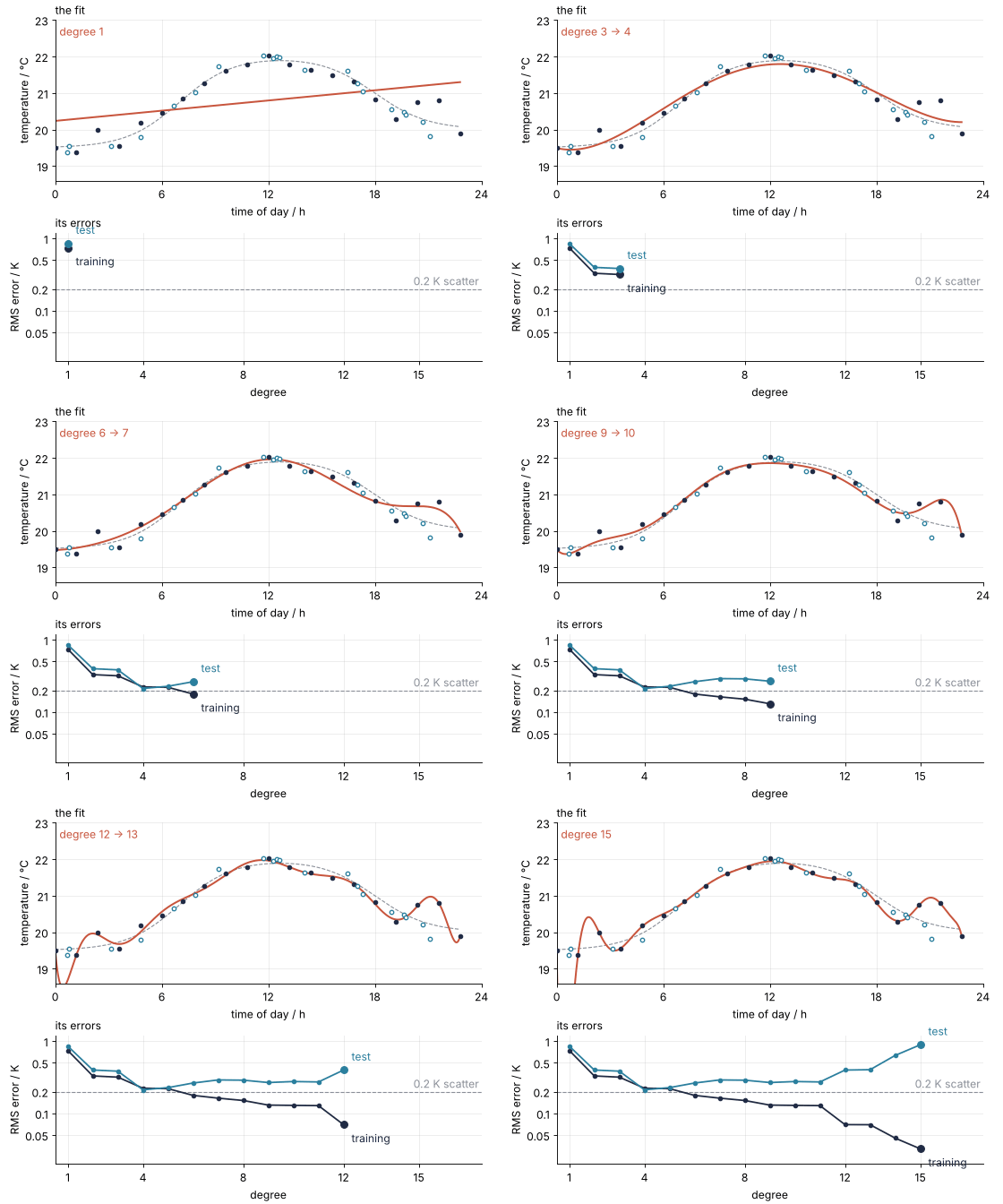
Animation. Top: temperature in °C against time of day, a polynomial fit going from degree 1 to 15 through filled readings, hollow fresh readings beside them. Bottom: training and test RMS error in K against degree. The training error keeps falling; the test error turns up after degree 4.

How I built this: each frame blends the fit of one degree into the next and extends both error curves by a point, with Matplotlib's FuncAnimation, the technique of Matplotlib animation with FuncAnimation; the source is animations/degree-sweep/scene.py.

Fresh readings and the U-shaped test curve

Show code

degrees = np.arange(1, 16)
fits = {d: Polynomial.fit(t_train, y_train, d) for d in degrees}
train_rms = np.array([rms(y_train - fits[d](t_train)) for d in degrees])
test_rms = np.array([rms(y_test - fits[d](t_test)) for d in degrees])
best = degrees[np.argmin(test_rms)]

print("degree   training / K   test / K")
for d, tr, te in zip(degrees, train_rms, test_rms):
    print(f"{d:6d}   {tr:12.3f}   {te:8.3f}")
print(f"lowest test error: degree {best}, {test_rms.min():.3f} K")

fig, ax = plt.subplots()
ax.axhline(SIGMA, color=MUTED, lw=1, ls="--")
ax.plot(degrees, train_rms, "o-", ms=4, color=INK)
ax.plot(degrees, test_rms, "o-", ms=4, color=SECOND)
ax.plot(best, test_rms.min(), "o", ms=8, color=ACCENT, zorder=3)
ax.annotate(f"degree {best}, {test_rms.min():.2f} K", (best, test_rms.min()), xytext=(10, 25),
            textcoords="offset points", color=ACCENT)
ax.text(15.3, train_rms[-1], "training", color=INK, va="center")
ax.text(15.3, test_rms[-1], "test", color=SECOND, va="center")
ax.text(15.3, SIGMA * 1.04, "0.2 K scatter", color=MUTED, va="bottom")
ax.set(xlabel="degree", ylabel="RMS error / K", yscale="log", xlim=(0.5, 18.5), xticks=[1, 4, 8, 12, 15])
ax.set_yticks([0.05, 0.1, 0.2, 0.5, 1], ["0.05", "0.1", "0.2", "0.5", "1"])
ax.minorticks_off()
plt.show()

degree   training / K   test / K
     1          0.746      0.855
     2          0.330      0.399
     3          0.317      0.384
     4          0.223      0.212
     5          0.220      0.227
     6          0.178      0.263
     7          0.162      0.290
     8          0.151      0.288
     9          0.130      0.267
    10          0.129      0.276
    11          0.128      0.272
    12          0.070      0.398
    13          0.070      0.403
    14          0.045      0.634
    15          0.032      0.891
lowest test error: degree 4, 0.212 K

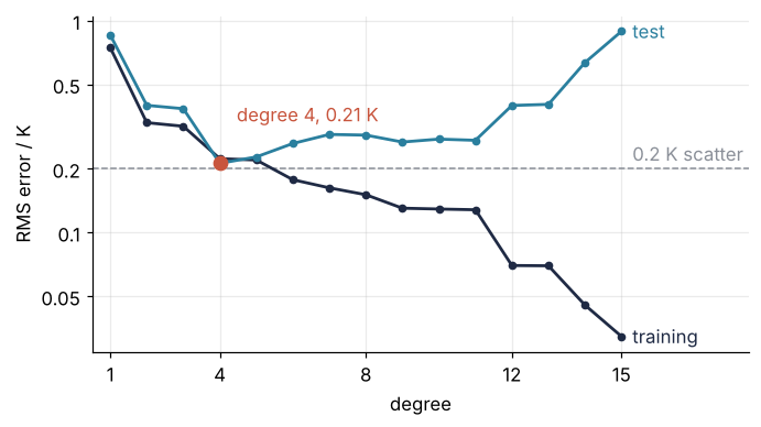
Training and test RMS error in K against polynomial degree 1 to 15, log scale, with the 0.2 K scatter dashed. The training error falls at every degree; the test error falls to 0.21 K at degree 4, marked, and rises to 0.89 K at degree 15.

The training error falls at every step, and it cannot do otherwise: a degree-5 polynomial can set its highest coefficient to zero and become the best degree-4 curve, so it never fits its own readings worse. The test error falls to 0.21 K at degree 4 and climbs back to 0.89 K at degree 15, a U. Left of the bottom the polynomial underfits, and right of the bottom it overfits. The bottom sits at the logger's 0.2 K, which no curve can beat, because the fresh readings scatter too. Degree 4 has learned the day and nothing else.

At degree 4 the two curves cross, and the test error is a little below the training error, 0.21 K against 0.22 K. That is luck: 20 fresh readings are a small sample with their own scatter, and degree 5 is only 0.015 K behind degree 4. The minimum of one test set is not sacred.

There is a catch in using the fresh readings this way. Picking degree 4 because it scored best on them made them part of the choice, so 0.21 K is now a flattering estimate of the error on readings still to come.

Formalization

A polynomial \(p_d\) of degree \(d\), fitted to \(N\) readings \((t_i, y_i)\), is scored by its root-mean-square misfit,

\[E(d) = \sqrt{\frac{1}{N}\sum_{i=1}^{N}\bigl(y_i - p_d(t_i)\bigr)^2} .\]

On the readings the fit used, \(E\) is the training error. On readings it did not use, the test set, it is the test error. Averaged over many training sets, it is the expected test error, which a choice of degree should minimize.

Training error always falls, as shown under the U-shaped curve. At \(d = N - 1 = 19\) the polynomial has as many coefficients as there are readings and passes through every one:

Show code

p19 = Polynomial.fit(t_train, y_train, N - 1)
print(f"degree 19 through 20 readings: training error {rms(y_train - p19(t_train)):.0e} K")
for d in [4, 15]:
    print(f"degree {d:2d}: expected training error {SIGMA * np.sqrt(1 - (d + 1) / N):.2f} K, "
          f"this draw {train_rms[d - 1]:.2f} K")

degree 19 through 20 readings: training error 4e-10 K
degree  4: expected training error 0.17 K, this draw 0.22 K
degree 15: expected training error 0.09 K, this draw 0.03 K

A training error of 4e-10 K is round-off: the fit is perfect on the readings it saw. Once the polynomial follows the true curve, only scatter is left, and each of the \(d + 1\) coefficients soaks up about one reading's share of it, so the expected squared training error is \(\sigma^2\,(1 - (d+1)/N)\), the count that Least squares derives as \(N - m\) for \(m\) coefficients, here \(m = d + 1\). For degree 4 that is 0.2 K · √(15/20) = 0.17 K against this draw's 0.22 K, and for degree 15 it is 0.09 K against 0.03 K: with four readings' worth of scatter left, single draws spread widely.

Bias and variance. The expected squared test error at a time \(t\) splits into three parts,

\[\bigl\langle (y - p_d(t))^2 \bigr\rangle = \text{bias}^2 + \text{variance} + \sigma^2 .\]

The bias is how far the average fit, over many training sets, lies from the true curve; the variance is how much single fits scatter around that average; \(\sigma^2\) is the fresh reading's own scatter, which no model removes. Here each degree is refitted on 1,000 training sets of 20 readings, both terms averaged over the day:

Show code

sim = np.random.default_rng(2026)
grid = np.linspace(0, T_END, 500)
R = 1000
refits = {d: np.empty((R, grid.size)) for d in degrees}
for r in range(R):
    y = truth(t_train) + SIGMA * sim.standard_normal(N)
    for d in degrees:
        refits[d][r] = Polynomial.fit(t_train, y, d)(grid)
bias2 = np.array([np.mean((refits[d].mean(axis=0) - truth(grid)) ** 2) for d in degrees])
variance = np.array([np.mean(refits[d].var(axis=0)) for d in degrees])

print("degree   bias² / K²   variance / K²")
for d in [1, 4, 15]:
    print(f"{d:6d}   {bias2[d - 1]:10.4f}   {variance[d - 1]:13.4f}")

fig, axes = plt.subplots(3, 1, figsize=(7, 6.6), sharex=True, sharey=True)
for ax, d in zip(axes, [1, 4, 15]):
    for r in range(30):
        ax.plot(grid, np.clip(refits[d][r], 17.5, 24.5), color=ACCENT, lw=1, alpha=0.25)
    ax.plot(grid, truth(grid), color=MUTED, lw=1.2, ls="--", zorder=3)
    ax.text(0.5, 0.96, f"degree {d}    bias² {bias2[d - 1]:.4f} K² · variance {variance[d - 1]:.4f} K²",
            transform=ax.transAxes, va="top", ha="center")
axes[1].set_ylabel("temperature / °C")
axes[-1].set(xlabel="time of day / h", xlim=(0, 24), xticks=[0, 6, 12, 18, 24], ylim=(18.6, 23.4))
plt.show()

degree   bias² / K²   variance / K²
     1       0.5871          0.0039
     4       0.0036          0.0088
    15       0.0001          0.3845

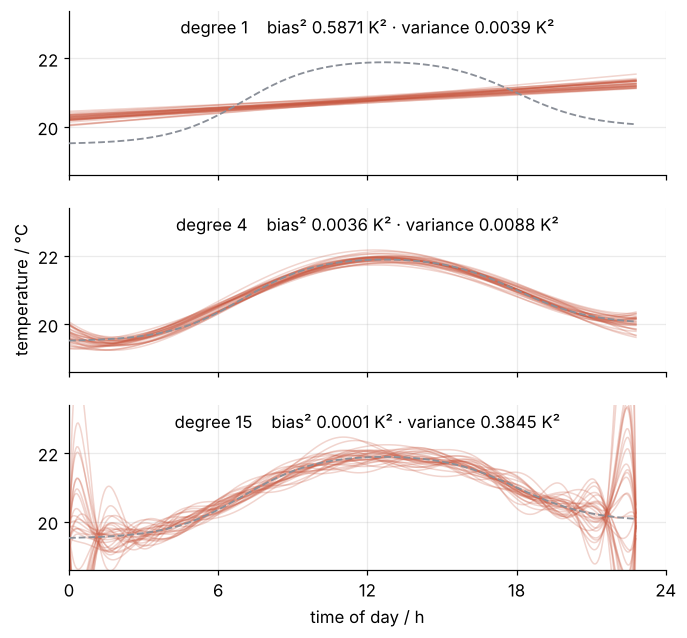
Three panels, temperature in °C against time of day, for degrees 1, 4, and 15, each with 30 fits to different draws of 20 readings and the dashed true curve. Degree 1: tight bundle, wrong shape. Degree 4: tight bundle on the curve. Degree 15: centered on the curve but spread wide.

Degree 1 is wrong the same way every time, bias² 0.59 K² and variance 0.004 K². Degree 15 is right on average, bias² 0.0001 K², and wrong every time, variance 0.38 K². Degree 4 keeps both small, 0.004 and 0.009 K², which is the bottom of the U.

More readings shrink the variance as \(\sigma^2 (d+1)/N\), but only while \(d + 1\) is well below \(N\): for degree 4 that gives 0.010 K² against 0.009 K² simulated, for degree 15 0.03 K² against 0.38 K². The bias does not depend on \(N\), so with more readings a higher degree pays. The curves below need no simulation: least squares is linear in the readings, so the average fit is the fit to the noiseless curve, and the variance is error propagation through each reading's weight in the fit.

Show code

def expected_test_rms(n):
    """Expected test RMS at each degree for n evenly spaced readings, without simulation."""
    t_n = np.linspace(0, T_END, n)
    out = []
    for d in degrees:
        b2 = np.mean((Polynomial.fit(t_n, truth(t_n), d)(grid) - truth(grid)) ** 2)
        weights = np.array([Polynomial.fit(t_n, e, d)(grid) for e in np.eye(n)])   # reading i's weight at each t
        var = SIGMA**2 * np.mean(np.sum(weights**2, axis=0))
        out.append(np.sqrt(b2 + var + SIGMA**2))
    return np.array(out)

expected = {n: expected_test_rms(n) for n in [20, 80, 320]}
simulated = np.sqrt(bias2 + variance + SIGMA**2)
print(f"check, 20 readings: exact and simulated agree to {np.max(np.abs(expected[20] / simulated - 1)):.1%}")
for n, e in expected.items():
    flat = degrees[e <= e.min() + 0.001]
    print(f"{n:3d} readings: lowest at degree {degrees[np.argmin(e)]:2d}, {e.min():.3f} K; "
          f"within 0.001 K: degrees {flat[0]} to {flat[-1]}")

from matplotlib.colors import to_rgb
# the test error keeps SECOND, lighter for fewer readings: mixed with white, so overlapping marks do not darken
tint = {n: tuple(1 - a * (1 - np.array(to_rgb(SECOND)))) for n, a in zip(expected, [0.5, 0.75, 1.0])}
fig, (top, zoom) = plt.subplots(2, 1, figsize=(7, 4.6), sharex=True)
for ax in (top, zoom):
    ax.axhline(SIGMA, color=MUTED, lw=1, ls="--")
    for n, e in expected.items():
        ax.plot(degrees, e, "o-", ms=4, color=tint[n])
        ax.plot(degrees[np.argmin(e)], e.min(), "o", ms=8, color=ACCENT, zorder=3)   # the best degree, red as in the U-shaped curve
top.text(15.3, expected[20][-1], "20 readings", color=tint[20], va="center")
top.set(yscale="log", ylim=(0.19, 0.9))
top.set_yticks([0.2, 0.3, 0.5, 0.8], ["0.2", "0.3", "0.5", "0.8"])
top.minorticks_off()
zoom.text(6.5, expected[20][5] - 0.003, "20 readings", color=tint[20], ha="center", va="top")
zoom.text(15.3, expected[80][-1], "80 readings", color=tint[80], va="center")
zoom.text(15.3, expected[320][-1], "320 readings", color=tint[320], va="center")
zoom.text(0.7, SIGMA + 0.0005, "0.2 K scatter", color=MUTED, va="bottom")
zoom.set(xlabel="degree", ylim=(0.198, 0.245), xlim=(0.5, 18.5), xticks=[1, 4, 8, 12, 15])
fig.supylabel("expected test RMS / K", fontsize=11)
plt.show()

check, 20 readings: exact and simulated agree to 0.6%
 20 readings: lowest at degree  4, 0.229 K; within 0.001 K: degrees 4 to 4
 80 readings: lowest at degree  9, 0.212 K; within 0.001 K: degrees 7 to 10
320 readings: lowest at degree 10, 0.204 K; within 0.001 K: degrees 9 to 14

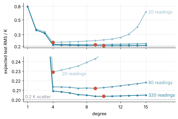
Expected test RMS error in K against degree for 20, 80, and 320 readings over the same day, log scale, in shades of blue from light to dark with each minimum in red, and the 0.2 K scatter dashed. The minimum moves from degree 4 to 9 to 10; the bottoms for 80 and 320 readings are flat over several degrees.

The minimum sits at degree 4 for 20 readings, at 9 for 80, and at 10 for 320. The last two bottoms are flat, degrees 7 to 10 and 9 to 14 within 0.001 K. The minimum barely moves from 80 to 320 readings because bias² is below 0.001 K² from degree 8 on.

Cross-validation. The U-shaped curve spent the fresh readings on choosing the degree. Readings used to choose are called a validation set; a test set is touched once, for the final report. 5-fold cross-validation makes validation sets out of the training readings themselves: shuffle the 20 readings into five groups of four, fit on 16, score on the other four, five times, and take the root of the mean of the 20 squared errors.

Show code

perm = rng.permutation(N)
folds = np.array_split(perm, 5)
cv_miss = np.empty((degrees.size, N))                # each reading's miss while it was held out
for k, d in enumerate(degrees):
    for fold in folds:
        keep = np.setdiff1d(np.arange(N), fold)
        p = Polynomial.fit(t_train[keep], y_train[keep], d)
        cv_miss[k, fold] = y_train[fold] - p(t_train[fold])
cv_rms = np.sqrt(np.mean(cv_miss ** 2, axis=1))      # average first, then the square root

print("degree   cross-validation / K   test / K")
for d in [1, 2, 3, 4, 5, 6, 7, 8, 15]:
    print(f"{d:6d}   {cv_rms[d - 1]:20,.2f}   {test_rms[d - 1]:8.2f}")
best_cv = degrees[np.argmin(cv_rms)]
miss = cv_miss[best_cv - 1]
print(f"cross-validation picks degree {best_cv}")
print(f"  the reading at {t_train[-1]:.1f} h, beyond its fit's data, missed by {abs(miss[-1]):.2f} K; "
      f"without the two end readings {rms(miss[1:-1]):.2f} K")

degree   cross-validation / K   test / K
     1                   0.91       0.86
     2                   0.39       0.40
     3                   0.38       0.38
     4                   0.37       0.21
     5                   0.53       0.23
     6                   0.65       0.26
     7                   0.84       0.29
     8                   1.78       0.29
    15               6,411.57       0.89
cross-validation picks degree 4
  the reading at 22.8 h, beyond its fit's data, missed by 1.17 K; without the two end readings 0.27 K

It picks degree 4, as the fresh readings did, from the 20 training readings alone. The bottom is flat, degrees 2 to 4 within 0.02 K. Its 0.37 K sits above the fresh readings' 0.21 K and is not your prediction error. Each fit sees 16 readings, not 20, and the folds holding out an end reading extrapolate: the reading at 22.8 h is missed by 1.17 K, and without the two end readings the cross-validation error is 0.27 K. Cross-validation is for choosing: where its minimum lies counts, not its height.

On your own data the test set comes out of your readings. Before fitting anything, set a fifth of them aside at random and do not look at them: of 25 readings, 5. Choose the degree by cross-validation on the other 20, refit on those 20 with that degree, and report the error on the 5 set-aside readings once, at the end. Classification with scikit-learn applies the same rule to the depth of a decision tree.

See it in code

scikit-learn does the cross-validation in one call, cross_val_score. A pipeline rescales the times to the range −1 to 1, builds the powers, and fits a linear model. The cell runs the scan twice. The first run uses the five shuffled folds of the loop above, so the two can be compared number by number. The second passes cv=5, which, like the default cv=None, cuts the readings into five blocks in time order:

Show code

from sklearn.pipeline import make_pipeline
from sklearn.preprocessing import MinMaxScaler, PolynomialFeatures
from sklearn.linear_model import LinearRegression
from sklearn.model_selection import cross_val_score

X = t_train.reshape(-1, 1)
splits = [(np.setdiff1d(np.arange(N), fold), fold) for fold in folds]

def cv_scan(cv):
    """Cross-validated RMS in K for degrees 1 to 10."""
    out = []
    for d in range(1, 11):
        model = make_pipeline(MinMaxScaler((-1, 1)), PolynomialFeatures(d), LinearRegression())
        mse = -cross_val_score(model, X, y_train, cv=cv, scoring="neg_mean_squared_error")
        out.append(np.sqrt(mse.mean()))
    return np.array(out)

sk_rms = cv_scan(splits)
print("degree   " + " ".join(f"{d:6d}" for d in range(1, 11)))
print("RMS / K  " + " ".join(f"{v:6.2f}" for v in sk_rms))
print(f"chosen degree {np.argmin(sk_rms) + 1}; largest difference from the NumPy loop {np.max(np.abs(sk_rms - cv_rms[:10])):.0e} K")
print(f"with cv=5, five unshuffled folds as by default: chosen degree {np.argmin(cv_scan(5)) + 1}")

degree        1      2      3      4      5      6      7      8      9     10
RMS / K    0.91   0.39   0.38   0.37   0.53   0.65   0.84   1.78   1.26   8.33
chosen degree 4; largest difference from the NumPy loop 1e-12 K
with cv=5, five unshuffled folds as by default: chosen degree 2

The first scan agrees with the NumPy loop to round-off, and both agree with the truth: the expected test error for 20 readings, computed from the known curve, is lowest at degree 4.

The second scan picks degree 2. Its contiguous blocks each remove almost five hours of the day and ask the fit to bridge the gap or, at the ends, to extrapolate past it. For interpolation within the span, as here, pass shuffled folds, KFold(5, shuffle=True, random_state=0), or your own; for forecasting forward in time, TimeSeriesSplit keeps the order and validates on later readings only. The scaler is not decoration. Polynomial.fit quietly rescales the times to −1 to 1 before fitting, and without that the fifteenth power of 22.8 h is about 10²⁰ and the fit loses its digits to round-off.

Where it shows up

Physics and engineering: calibration curves. A thermocouple or a resistance thermometer is often calibrated with a polynomial in its reading. Choose the degree by the error on check points left out of the fit, not by the residuals of the points in it, or every later measurement inherits the noise of the calibration run.
Chemistry and physics: spectral baselines. A polynomial baseline under a Raman, IR, or X-ray photoelectron spectrum must follow the slow background and nothing else, and too high a degree bends up into the peaks and eats part of their area. The number of peaks in a multi-peak fit is the same choice: one more peak always lowers the residuals.
Particle physics: signal and background. A classifier that sorts detector events into signal and background overfits like the polynomial. The decision tree in Classification with scikit-learn, at its default depth, scores 100 % on its 1,500 training events and 75.4 % on 500 held-out ones, and its depth, chosen there by cross-validation, plays the role of the degree.
Biology and medicine: gene-expression models. A study of a few hundred patients with thousands of measured genes hands a model more parameters than samples, and such a model can fit its training patients perfectly unless held-out data or a penalty stops it. A neural network is often stopped early: training halts when the error on a validation set starts to rise.
Statistics: information criteria. AIC and BIC add a penalty for every parameter to the training misfit. They stand in for held-out data when there are too few readings to spare any.
Geophysics: inversions. A seismic or gravity inversion with Tikhonov damping trades variance for bias through its damping parameter, so choosing that parameter is choosing the degree. Generalized cross-validation, a fast relative of the procedure above, is one of the standard ways to pick it.

In every case the knob is a count of parameters or the strength of a penalty, and the fit's own residuals alone cannot set it.

The question

The idea: a flexible curve fits the noise too

Fresh readings and the U-shaped test curve

Formalization

See it in code

Where it shows up

Further reading