Bootstrap confidence intervals with scipy.stats: the median grain size of sand

The problem: how well forty samples pin down the median grain size

A geologist takes forty sand samples across one river bar and runs each through a laser diffraction analyzer. Most come out as fine to medium sand around 0.3 mm, a handful as coarse sand, and one at 2.06 mm. The report needs the median grain size, which sedimentologists call the D50, with a 95 % confidence interval. The median of the forty is 0.3065 mm, and the bootstrap, run through scipy.stats.bootstrap, puts it between 0.2225 and 0.4385 mm: 0.084 mm below and 0.132 mm above, lopsided like the sand itself.

Why not a formula? s/√n is the standard error of the mean, not of the median. Textbooks give the median one too, 1.2533 s/√n, but it assumes normally distributed data, and this sand is not normal. For most other statistics, such as a ratio of two medians, a correlation of skewed data, or the D84, the size that 84 % of the sample is finer than, there is no formula at hand. The bootstrap gives an interval for every one of them with the same call. A biologist reads the forty values as body masses or cell volumes, an engineer as the particle sizes of a powder; from here on they are grain sizes.

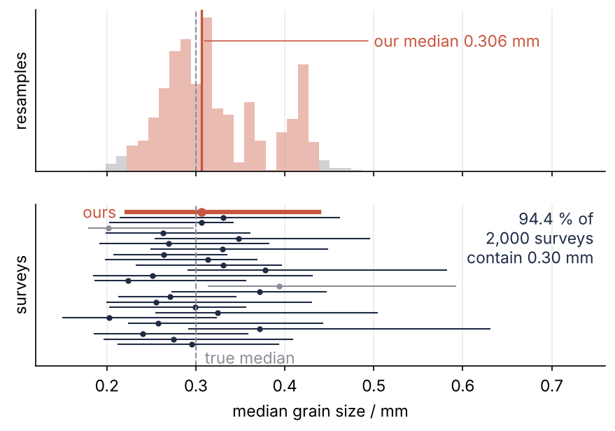
The top panel is the bootstrap's picture of where our median could have landed, with its 95 % interval in red. The bottom panel tests the procedure on 2,000 fresh surveys of the same bar, whose true median of 0.30 mm is known because the data are simulated, and 94.4 % of the intervals contain it. The textbook formula's intervals contain it 99.4 % of the time, which sounds better and is not: they are 63 % wider than they need to be. Step 5 draws the figure.

Setup

One seeded generator draws everything below: the forty grain sizes d, forty more from a bar 5 km downstream with a true median of 0.15 mm, and the flow velocity v at each sampling point of the first bar, built partly from the log grain size so that it runs faster where the grains are coarser.

import numpy as np
import matplotlib.pyplot as plt
from scipy import stats

# the true bar: unknown in a real survey; here it generates the data and checks the results (Steps 3 to 5)
median_true = 0.30                                    # mm
sigma_ln = 0.9                                        # spread of ln(grain size)
mean_true = median_true * np.exp(sigma_ln**2 / 2)     # 0.450 mm
median_down = 0.15                                    # mm, the bar 5 km downstream
n = 40                                                # samples per bar

rng = np.random.default_rng(42)
d = np.round(rng.lognormal(np.log(median_true), sigma_ln, n), 3)      # grain sizes, mm; analyzers report 1 µm
down = np.round(rng.lognormal(np.log(median_down), sigma_ln, n), 3)
z = (np.log(d) - np.log(d).mean()) / np.log(d).std()
v = np.round(0.6 + 0.15 * (0.6 * z + 0.8 * rng.standard_normal(n)), 2)  # flow velocity, m/s

plt.rcParams.update({
    "figure.figsize": (7, 3.6), "figure.dpi": 110,
    "axes.spines.top": False, "axes.spines.right": False,
    "axes.grid": True, "grid.alpha": 0.25,
    "font.size": 11, "lines.linewidth": 1.8,
})
INK, ACCENT, SECOND, MUTED = "#1f2a44", "#c8553d", "#2a7f9e", "#8a8f98"

print(f"n = {n}   median {np.median(d):.4f} mm   mean {d.mean():.3f} mm   sd {d.std(ddof=1):.3f} mm   "
      f"largest {d.max():.3f} mm   below the mean {100 * np.mean(d < d.mean()):.1f} %")

n = 40   median 0.3065 mm   mean 0.407 mm   sd 0.350 mm   largest 2.062 mm   below the mean 57.5 %

Step 1: Resample the forty values by hand

The sample is the best picture you have of the bar. Drawing forty values from it with replacement, some twice and some not at all, is a new survey you did not have to walk. The spread of the medians of 9,999 such surveys stands in for the spread of your median. That is the bootstrap. First the data:

Show code

Copy

fig, ax = plt.subplots(figsize=(7, 2.4))
jitter = np.random.default_rng(0).uniform(-0.3, 0.3, n)      # only spreads the dots vertically
ax.plot(d, jitter, "o", color=INK, ms=4)
for value, color, label, side in [(np.median(d), ACCENT, "median", "right"), (d.mean(), SECOND, "mean", "left")]:
    ax.axvline(value, color=color, lw=1.4)
    shift = -0.015 if side == "right" else 0.015
    ax.text(value + shift, 0.45, f"{label} {value:.3f} mm", color=color, ha=side, va="bottom")
ax.grid(axis="y", visible=False)
ax.spines["left"].set_visible(False)
ax.set(xlabel="grain size / mm", yticks=[], ylim=(-0.5, 0.7), xlim=(0, 2.2))
plt.show()

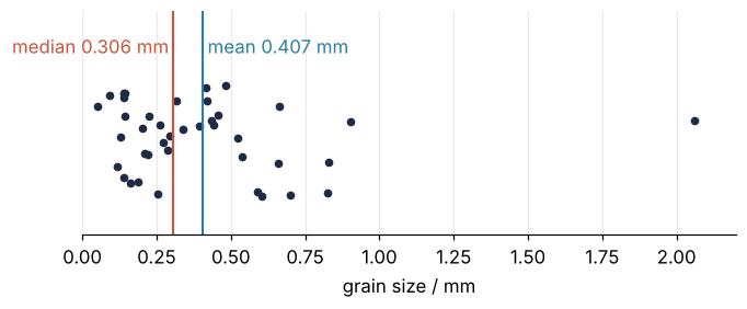
A handful of coarse grains pull the mean, 0.407 mm, above 57.5 % of the samples. Now the resampling, with rng.choice as in Random numbers with numpy.random:

resamples = rng.choice(d, size=(9999, n))       # 9,999 surveys, each 40 draws from our 40 values
medians = np.median(resamples, axis=1)
low, high = np.percentile(medians, [2.5, 97.5])
print(f"median {np.median(d):.4f} mm   95 % interval {low:.4f} to {high:.4f} mm")
print(f"bootstrap standard error of the median {medians.std(ddof=1):.3f} mm   "
      f"distinct values among the 9,999 medians: {len(np.unique(medians))}")

median 0.3065 mm   95 % interval 0.2225 to 0.4385 mm
bootstrap standard error of the median 0.062 mm   distinct values among the 9,999 medians: 125

The interval, 0.2225 to 0.4385 mm, runs from the 2.5th to the 97.5th percentile of the medians, and their standard deviation, 0.062 mm, is the bootstrap standard error of the median. The 9,999 medians take only 125 distinct values. A median of forty is the average of the 20th and 21st sorted values, and only a handful of original values near the middle ever land there, so those values and their pairwise averages are all that can occur.

Step 2: Let stats.bootstrap do it, with percentile and BCa

stats.bootstrap does the same and returns more. The data go in as a tuple of samples, (d,), because the same call takes two samples in Step 4. np.median accepts an axis argument, so SciPy evaluates all resamples in one array call. rng=rng makes the draws reproducible.

res_pct = stats.bootstrap((d,), np.median, method="percentile", rng=rng)
res = stats.bootstrap((d,), np.median, rng=rng)             # method="BCa", the default
for name, r in [("percentile", res_pct), ("BCa", res)]:
    ci = r.confidence_interval
    print(f"{name:10s} {ci.low:.4f} to {ci.high:.4f} mm   standard error {r.standard_error:.3f} mm")
print("bootstrap_distribution:", res.bootstrap_distribution.shape)

percentile 0.2225 to 0.4385 mm   standard error 0.061 mm
BCa        0.2225 to 0.4385 mm   standard error 0.061 mm
bootstrap_distribution: (9999,)

The result carries confidence_interval (low, high), standard_error, and bootstrap_distribution, the 9,999 medians themselves. The percentile interval is Step 1's, to the digit. The default, method="BCa" (bias-corrected and accelerated), adjusts it twice. The bias correction shifts both ends when the bootstrap distribution is not centered on the estimate. The acceleration stretches one side when the statistic scatters more on one side of its value than on the other. SciPy estimates it with the jackknife: compute the statistic forty times, each time on the sample with one value left out; the more lopsided those forty values, the larger the acceleration. For the median, both corrections come to nothing:

leave_one_out = np.array([np.median(np.delete(d, i)) for i in range(n)])
values, counts = np.unique(leave_one_out, return_counts=True)
print("leave-one-out medians:", values, "mm, counted", counts, "times")
boot = res.bootstrap_distribution
below = np.mean(boot < np.median(d)) + 0.5 * np.mean(boot == np.median(d))   # ties count half, as in SciPy
print(f"bootstrap medians below the estimate: {100 * below:.1f} %   distinct values among them: {len(np.unique(boot))}")

leave-one-out medians: [0.295 0.318] mm, counted [20 20] times
bootstrap medians below the estimate: 49.3 %   distinct values among them: 122

Leaving out a value below the middle makes the 21st sorted value the median, 0.318 mm; leaving out one above makes it the 20th, 0.295 mm. Twenty times each is a perfectly symmetric set, so the acceleration is exactly zero.

The bias correction starts from the share of bootstrap medians below the estimate: 49.3 %, where a centered distribution gives 50 %. It turns that share into a normal quantile, z₀ = Φ⁻¹(0.493) = −0.018, with Φ the standard normal distribution function, and moves the cuts from Φ(∓1.96) to Φ(2z₀ ∓ 1.96), from the 2.5th and 97.5th percentiles to the 2.3rd and 97.3rd. SciPy drew its own 9,999 resamples, whose medians take 122 distinct values against the 125 of Step 1, and among so few distinct values a shift of 0.2 percentiles does not reach the next one. BCa ends on 0.2225 and 0.4385 mm, the ends of the percentile interval. Keep BCa anyway; Step 3 shows where it matters.

Last, the number of resamples:

for R in [99, 999, 9999]:
    lows = [stats.bootstrap((d,), np.median, n_resamples=R, rng=rng).confidence_interval.low for _ in range(5)]
    print(f"n_resamples = {R:5d}   lower bound in five runs: " + "  ".join(f"{x:.4f}" for x in lows) + " mm")

n_resamples =    99   lower bound in five runs: 0.2392  0.2211  0.2400  0.2252  0.2257 mm
n_resamples =   999   lower bound in five runs: 0.2260  0.2190  0.2225  0.2347  0.2246 mm
n_resamples =  9999   lower bound in five runs: 0.2225  0.2225  0.2225  0.2225  0.2225 mm

With 99 resamples the lower bound wanders by 0.019 mm from run to run, with 999 still by 0.016 mm, and with 9,999 it does not move. Keep the default.

Step 3: Compare with the textbook formulas

The textbook interval for a median rests on one fact about normal data: there the standard error of the median is √(π/2) ≈ 1.2533 times that of the mean, s/√n. The formula borrows the sample standard deviation s and the normal shape, and gives median ± 1.96 × 1.2533 s/√n:

m = np.median(d)
half = 1.96 * np.sqrt(np.pi / 2) * d.std(ddof=1) / np.sqrt(n)
ci = res.confidence_interval
print(f"formula   {m - half:.4f} to {m + half:.4f} mm   reaches {half:.3f} below and {half:.3f} above")
print(f"bootstrap {ci.low:.4f} to {ci.high:.4f} mm   reaches {m - ci.low:.3f} below and {ci.high - m:.3f} above")

formula   0.1707 to 0.4423 mm   reaches 0.136 below and 0.136 above
bootstrap 0.2225 to 0.4385 mm   reaches 0.084 below and 0.132 above

The formula reaches 0.136 mm on either side, the bootstrap 0.084 mm below and 0.132 mm above: below the median the formula reaches 62 % further. To see why, double the largest grain in a copy of the data, and give both bootstrap calls the same seed so that they draw the same resamples.

d2 = d.copy()
d2[np.argmax(d2)] *= 2                          # the coarsest grain, twice as coarse
for name, x in [("as measured", d), ("largest doubled", d2)]:
    same = np.random.default_rng(1)             # the same seed for both: the same resamples
    ci_x = stats.bootstrap((x,), np.median, rng=same).confidence_interval
    half_x = 1.96 * np.sqrt(np.pi / 2) * x.std(ddof=1) / np.sqrt(n)
    print(f"{name:15s}  median {np.median(x):.4f}  s {x.std(ddof=1):.3f}  formula ± {half_x:.3f}  "
          f"bootstrap {ci_x.low:.4f} to {ci_x.high:.4f} mm")

as measured      median 0.3065  s 0.350  formula ± 0.136  bootstrap 0.2225 to 0.4385 mm
largest doubled  median 0.3065  s 0.635  formula ± 0.247  bootstrap 0.2225 to 0.4385 mm

The median and the bootstrap interval do not move, while s rises from 0.350 to 0.635 mm and the formula's half-width from 0.136 to 0.247 mm. s follows the coarse tail; the error of the median depends only on how densely the values crowd around the middle. The formula ties one to the other through a normal shape the sand does not have.

The mean has its own textbook interval, the t-interval from Step 2 of scipy.stats from the ground up. Against the bootstrap:

t_low, t_high = stats.t.interval(0.95, df=n - 1, loc=d.mean(), scale=stats.sem(d))
mean_pct = stats.bootstrap((d,), np.mean, method="percentile", rng=rng)
mean_bca = stats.bootstrap((d,), np.mean, rng=rng)
print(f"mean {d.mean():.3f} mm")
print(f"t-interval  {t_low:.3f} to {t_high:.3f} mm")
for name, r in [("percentile", mean_pct), ("BCa", mean_bca)]:
    print(f"{name:11s} {r.confidence_interval.low:.3f} to {r.confidence_interval.high:.3f} mm")

mean 0.407 mm
t-interval  0.295 to 0.519 mm
percentile  0.313 to 0.526 mm
BCa         0.329 to 0.559 mm

Show code

Copy

fig, ax = plt.subplots(figsize=(7, 3.2))
counts_m, edges_m, _ = ax.hist(mean_bca.bootstrap_distribution, bins=60, color=MUTED, lw=0, alpha=0.6)
x = np.linspace(edges_m[0], edges_m[-1], 300)
scale = len(mean_bca.bootstrap_distribution) * (edges_m[1] - edges_m[0])   # density to counts per bin
ax.plot(x, scale * stats.t.pdf(x, df=n - 1, loc=d.mean(), scale=stats.sem(d)), color=SECOND, lw=1.4)
top_y = counts_m.max()
lo_b, hi_b = mean_bca.confidence_interval
ax.plot([lo_b, hi_b], [-0.08 * top_y] * 2, color=ACCENT, lw=4, solid_capstyle="butt")
ax.plot([t_low, t_high], [-0.18 * top_y] * 2, color=SECOND, lw=4, solid_capstyle="butt")
ax.text(hi_b + 0.01, -0.08 * top_y, "BCa", color=ACCENT, va="center")
ax.text(t_high + 0.01, -0.18 * top_y, "t", color=SECOND, va="center")
ax.axvline(mean_true, color=MUTED, lw=1, ls="--")
ax.text(mean_true + 0.005, 0.95 * top_y, "true mean", color=MUTED, va="top")
ax.set(xlabel="mean grain size / mm", ylabel="resamples", yticks=[], ylim=(-0.25 * top_y, 1.05 * top_y))
plt.show()

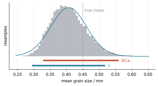
The bootstrap means lean right, like the grain sizes; the t curve does not. BCa follows the lean and, unlike for the median, departs from the percentile interval: it sits 0.034 mm higher at the bottom and 0.041 mm higher at the top than the symmetric t-interval. All three contain the true mean, 0.450 mm. Which method holds its 95 % is for Step 5.

Step 4: Bootstrap two samples and paired values

The ratio of the median grain sizes of the two bars says how much the sand fines over 5 km. The statistic takes one argument per sample, plus axis:

def ratio_of_medians(x, y, axis):
    return np.median(x, axis=axis) / np.median(y, axis=axis)

ratio = stats.bootstrap((d, down), ratio_of_medians, rng=rng)
print(f"median downstream {np.median(down):.4f} mm   ratio {ratio_of_medians(d, down, -1):.2f}   "
      f"95 % interval {ratio.confidence_interval.low:.2f} to {ratio.confidence_interval.high:.2f}")

median downstream 0.1720 mm   ratio 1.78   95 % interval 1.15 to 2.91

SciPy resamples each sample on its own, forty values from each bar. The upstream bar is coarser by a factor of 1.78, somewhere between 1.15 and 2.91, and the true 2.0 lies inside. The interval excludes 1, so the fining is real. It reaches 0.63 below the estimate and 1.13 above: a ratio is bounded by zero below and by nothing above.

Paired values are a different case. Each velocity in v belongs to the grain size at the same point, and paired=True resamples whole sampling points, the same indices into both arrays. The correlation uses the logarithm of grain size, which spreads by factors (Pitfall 2 of the prerequisite):

def log_corr(x, y, axis):
    return stats.pearsonr(np.log(x), y, axis=axis).statistic

corr = stats.bootstrap((d, v), log_corr, paired=True, rng=rng)
print(f"r = {log_corr(d, v, -1):.3f}   95 % interval {corr.confidence_interval.low:.3f} to "
      f"{corr.confidence_interval.high:.3f}")

r = 0.719   95 % interval 0.479 to 0.865

Coarse grains lie where the current runs faster, with r = 0.719 and an interval from 0.479 to 0.865. It reaches 0.240 below the estimate and only 0.146 above, because a correlation cannot exceed 1.

Step 5: Check the coverage on 2,000 fresh surveys

Draw 2,000 new surveys of forty values from the true bar of the Setup, one per row, and axis=-1 puts an interval on every row in one call. 2,000 resamples suffice, because the share of hits is measured, not each interval; batch=100 computes them a hundred at a time, 64 MB at once. The table adds a fourth median interval that needs no resampling, the 14th to the 27th sorted value, explained below. The cell is slow.

surveys = rng.lognormal(np.log(median_true), sigma_ln, (2000, n))     # one survey per row
fast = dict(axis=-1, n_resamples=2000, batch=100, rng=rng)
m_s = np.median(surveys, axis=-1)
half_s = 1.96 * np.sqrt(np.pi / 2) * surveys.std(ddof=1, axis=-1) / np.sqrt(n)
median_bca = stats.bootstrap((surveys,), np.median, **fast).confidence_interval
intervals = {
    "median, percentile": (stats.bootstrap((surveys,), np.median, method="percentile", **fast).confidence_interval,
                           median_true),
    "median, BCa": (median_bca, median_true),
    "median, formula": ((m_s - half_s, m_s + half_s), median_true),
    "median, 14th to 27th": (tuple(np.sort(surveys, axis=-1)[:, [13, 26]].T), median_true),
    "mean, t": (stats.t.interval(0.95, df=n - 1, loc=surveys.mean(axis=-1), scale=stats.sem(surveys, axis=-1)),
                mean_true),
    "mean, BCa": (stats.bootstrap((surveys,), np.mean, **fast).confidence_interval, mean_true),
}
print(f"{'':21s}{'contains':>9s}{'too low':>10s}{'too high':>10s}{'width':>11s}")
for name, ((lo, hi), truth) in intervals.items():
    print(f"{name:21s}{100 * np.mean((lo <= truth) & (truth <= hi)):7.1f} %{100 * np.mean(hi < truth):8.1f} %"
          f"{100 * np.mean(lo > truth):8.1f} %{np.median(hi - lo):8.3f} mm")

                      contains   too low  too high      width
median, percentile      94.7 %     2.8 %     2.5 %   0.205 mm
median, BCa             94.4 %     3.0 %     2.6 %   0.203 mm
median, formula         99.4 %     0.2 %     0.4 %   0.332 mm
median, 14th to 27th    95.9 %     2.1 %     2.0 %   0.225 mm
mean, t                 91.3 %     8.3 %     0.4 %   0.273 mm
mean, BCa               91.6 %     5.8 %     2.6 %   0.274 mm

A coverage from 2,000 surveys carries a Monte Carlo error of √(p(1 − p)/N) = √(0.95 × 0.05 / 2000) ≈ 0.005, half a percentage point (Monte Carlo integration says why), so the bootstrap's 94.4 and 94.7 % lie within about one such error of 95 %, with misses on both sides ("too low" is an interval entirely below the truth). The formula reaches 99.4 % by being 63 % wider than BCa, 0.332 against 0.203 mm.

For the mean, nothing reaches 95 %. The t-interval misses almost only low, because a survey that caught few coarse grains has a low mean and a small s at once, and BCa's 91.6 % is within the noise of the t-interval's 91.3 %. For the mean of a skewed quantity at forty samples, the bootstrap is not a repair.

On your own data the sample shows when it is not normal: a mean further above the median than SciPy's standard error of the median (here 0.407 against 0.3065 mm, with 0.061 mm), or a bootstrap interval clearly lopsided about the estimate (here 0.084 mm below, 0.132 mm above). For a median, either sign means: report the bootstrap interval, not the formula. For a mean, it means neither interval holds its 95 %: take more samples, or say so.

The row "14th to 27th" holds for any continuous distribution. Each value falls below the true median with probability one half, so the count below it is binomial with p = 0.5, and 13 or fewer fall below in under 2.5 % of samples: the 14th sorted value is the lower end. By symmetry the upper end is the 14th from the top, the 27th:

k = int(stats.binom.ppf(0.025, n, 0.5))         # the count of values below the true median is binomial(40, 1/2)
lo_os, hi_os = np.sort(d)[[k - 1, n - k]]
level = stats.binom.cdf(n - k, n, 0.5) - stats.binom.cdf(k - 1, n, 0.5)
print(f"values {k} and {n + 1 - k} of the sorted sample: {lo_os:.3f} to {hi_os:.3f} mm, "
      f"coverage {100 * level:.1f} % for any continuous distribution")

values 14 and 27 of the sorted sample: 0.219 to 0.442 mm, coverage 96.2 % for any continuous distribution

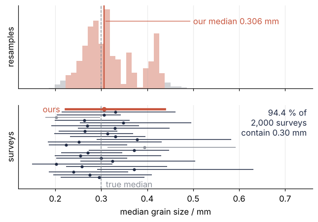
It lies within 0.004 mm of the bootstrap interval at both ends and 0.048 mm above the formula's lower end: trust the interval that agrees with it. The final figure puts ours among the first 25 surveys:

Copy

fig, (top, bottom) = plt.subplots(2, 1, figsize=(7, 4.4), sharex=True)

# top: the bootstrap distribution of our median, with bin edges a hair outside the interval ends
lo, hi = res.confidence_interval
w = (hi - lo + 2e-9) / 18
edges = (lo - 1e-9) + w * np.arange(-8, 30)
counts_b, _ = np.histogram(res.bootstrap_distribution, edges)
centers = edges[:-1] + w / 2
inside = (centers > lo) & (centers < hi)
top.bar(centers, counts_b, width=w, lw=0, color=np.where(inside, ACCENT, MUTED), alpha=0.4)
top.axvline(np.median(d), color=ACCENT, lw=1.6)
top.annotate(f"our median {np.median(d):.3f} mm", (np.median(d), 0.85 * counts_b.max()),
             xytext=(0.5, 0.85 * counts_b.max()), color=ACCENT, va="center",
             arrowprops=dict(arrowstyle="-", color=ACCENT, lw=0.8))
top.set(ylabel="resamples", yticks=[])

# bottom: our interval on top, then the BCa intervals of the first 25 fresh surveys
rows = np.arange(1, 26)
lo25, hi25 = median_bca.low[:25], median_bca.high[:25]
hit = (lo25 <= median_true) & (median_true <= hi25)
bottom.plot([lo, hi], [0, 0], color=ACCENT, lw=3)
bottom.plot(np.median(d), 0, "o", color=ACCENT, ms=5)
bottom.text(lo - 0.012, 0, "ours", color=ACCENT, ha="right", va="center")
for mask, color in [(hit, INK), (~hit, MUTED)]:
    bottom.hlines(rows[mask], lo25[mask], hi25[mask], color=color, lw=1)
    bottom.plot(m_s[:25][mask], rows[mask], "o", color=color, ms=3)
for ax in (top, bottom):
    ax.axvline(median_true, color=MUTED, lw=1, ls="--")
lo_all, hi_all = median_bca
coverage = 100 * np.mean((lo_all <= median_true) & (median_true <= hi_all))
bottom.text(median_true + 0.01, 27.5, "true median", color=MUTED, va="center")
bottom.text(0.98, 0.97, f"{coverage:.1f} % of\n2,000 surveys\ncontain {median_true:.2f} mm", color=INK, ha="right", va="top",
            transform=bottom.transAxes)
bottom.set(xlabel="median grain size / mm", ylabel="surveys", yticks=[], xlim=(0.12, 0.76), ylim=(29, -1.5))
plt.show()

Pitfalls

Breaking the pairs. Leave out paired=True in Step 4 and the default BCa stops with ValueError: `x` and `y` must be broadcastable. The jackknife of Step 2 leaves out one value from one sample at a time, so 39 grain sizes meet 40 velocities. That error is the lucky case. With method="percentile" there is no jackknife, and the call runs:

unpaired = stats.bootstrap((d, v), log_corr, method="percentile", rng=rng)
print(f"without paired=True: {unpaired.confidence_interval.low:.2f} to {unpaired.confidence_interval.high:.2f}")

without paired=True: -0.31 to 0.32

An interval from −0.31 to 0.32 around zero, for a correlation of 0.719. Resampling the two arrays independently pairs each grain size with a random velocity and destroys the correlation the interval was meant to measure. Set paired=True whenever the values belong together.

A sample too small. The bootstrap only knows the values you have. With ten samples per survey, over 1,000 surveys:

small = rng.lognormal(np.log(median_true), sigma_ln, (1000, 10))       # 1,000 surveys of ten samples
fast = dict(axis=-1, n_resamples=2000, batch=100, rng=rng)
for name, statistic, truth in [("median, BCa", np.median, median_true), ("mean, BCa", np.mean, mean_true)]:
    r = stats.bootstrap((small,), statistic, **fast)
    lo, hi = r.confidence_interval
    print(f"{name:12s} contains the truth in {100 * np.mean((lo <= truth) & (truth <= hi)):4.1f} %   "
          f"median width {np.median(hi - lo):.3f} mm   distinct values in one bootstrap distribution: "
          f"{len(np.unique(r.bootstrap_distribution[0]))}")

median, BCa  contains the truth in 93.9 %   median width 0.422 mm   distinct values in one bootstrap distribution: 37
mean, BCa    contains the truth in 83.7 %   median width 0.425 mm   distinct values in one bootstrap distribution: 1960

The median interval still contains the truth in 93.9 % of surveys, but it is 0.422 mm wide, twice the 0.203 mm at forty, and built from 37 distinct bootstrap medians. The mean's BCa interval drops to 83.7 %, because ten values rarely include the coarse tail that sets the mean. Take more samples. If you cannot, report the order-statistic interval of Step 5, which at ten values is the 2nd to the 9th sorted value with 97.9 % coverage, and say that the interval is rough.

A sample that is not representative. Forty samples all taken from the coarse head of the bar give a tight interval around the wrong median, and no number of resamples moves it. The bootstrap measures the scatter of sampling, not its bias. The fix is the sampling design, a grid or random positions across the whole bar, decided before the field day.

Variations

• Any percentile, such as the D84. Pass lambda x, axis: np.percentile(x, 84, axis=axis) as the statistic; the D84 sets the bed roughness in hydraulics.
• Sorting in phi units. -np.log2(x) turns millimeters into the Krumbein phi scale, and the standard deviation in phi is what sedimentologists call sorting: bootstrap lambda x, axis: np.std(-np.log2(x), axis=axis, ddof=1).
• A one-sided bound. alternative="less" returns an upper limit only, with the lower end at minus infinity, for a specification such as "median below 0.5 mm".
• A statistic without an axis argument. vectorized=False makes bootstrap call any function of one sample, a fit or a hand-written estimator, one resample at a time. It is correct, but the function runs once on the sample, once per resample, and once per left-out value for the BCa jackknife: 10,040 calls for forty values at the default, so a fit that takes 10 ms costs well over a minute. Start with n_resamples=999.

Cheat sheet

res = stats.bootstrap((x,), np.median, rng=rng)        # data as a tuple; BCa, 9,999 resamples by default
res.confidence_interval.low, res.confidence_interval.high, res.standard_error
res.bootstrap_distribution                             # the statistic on every resample
stats.bootstrap((x,), np.median, method="percentile")  # plain percentiles of the resamples
def f(x, y, axis):                                     # a statistic: one argument per sample, plus axis
    return np.median(x, axis=axis) / np.median(y, axis=axis)
stats.bootstrap((x, y), f)                             # two samples, each resampled on its own
stats.bootstrap((x, y), g, paired=True)                # pairs stay together; needed for correlations
stats.bootstrap((X,), np.median, axis=-1, batch=100)   # one interval per row of X; batch caps memory

Further reading

• The scipy.stats.bootstrap reference, with the three methods and the bootstrap_result argument for adding resamples to an earlier run.
• Bradley Efron and Robert J. Tibshirani, An Introduction to the Bootstrap (Chapman & Hall, 1993), where BCa is derived, and A. C. Davison and D. V. Hinkley, Bootstrap Methods and Their Application (Cambridge University Press, 1997), for the cases where the bootstrap fails.
• Related tutorials on this site: scipy.stats from the ground up: is the difference between two samples real?, for t-intervals and coverage by reruns; Uncertainty propagation by sampling with NumPy, which reports a skewed result as a median with a 95 % interval; The standard error of the mean; Monte Carlo integration; seaborn from the ground up, whose bar plots draw bootstrap intervals; planned: the same tutorial in Julia with Bootstrap.jl.
• Download the notebook. It was executed with the library versions in the header.