Rational approximation: why a resonance needs a ratio of polynomials

The question

A driven, damped oscillator with quality factor Q = 50 stands for a tuned LC circuit, a microwave cavity, or a spectral line. Scaled to a peak height of 1, its power response is

with ω in units of the resonance frequency ω₀. On [0, 2] that is one smooth bump, and the usual tool for approximating a smooth function on an interval is a polynomial. Rational approximation, with a ratio of two polynomials, is the less usual one. Here is the resonance next to the polynomial of degree 100 that matches it at 101 points:

Show code

Copy

import warnings

import numpy as np
import mpmath
import matplotlib.pyplot as plt
from numpy.polynomial import Chebyshev
from scipy.interpolate import AAA

plt.rcParams.update({
    "figure.figsize": (8, 3.2), "figure.dpi": 110,
    "axes.spines.top": False, "axes.spines.right": False,
    "axes.grid": True, "grid.alpha": 0.25,
    "font.size": 11, "lines.linewidth": 1.8,
})
INK, ACCENT, SECOND, MUTED = "#1f2a44", "#c8553d", "#2a7f9e", "#8a8f98"

Q = 50

def power(w, Q=Q):
    """Power response of a driven damped oscillator, peak height 1, w in units of w0."""
    return 1 / (Q**2 * ((1 - w**2) ** 2 + (w / Q) ** 2))

wf = np.linspace(0, 2, 40001)          # the fine grid every error is measured on
x = np.linspace(0, 2, 2000)            # the samples AAA gets: spacing 0.0010
Pf = power(wf)

def cheb_error(n, f=power):
    """Maximum error of the degree-n Chebyshev interpolant of f on [0, 2]."""
    c = Chebyshev.interpolate(f, n, domain=[0, 2])
    return np.max(np.abs(c(wf) - f(wf))), c

above = wf[Pf >= 0.5 * Pf.max()]
err100, c100 = cheb_error(100)
print(f"peak at ω = {wf[np.argmax(Pf)]:.5f} ω₀, width at half height {above[-1] - above[0]:.4f} ω₀")
print(f"degree-100 polynomial through 101 Chebyshev points: max error {err100:.2f} of the peak height")

fig, (ax1, ax2) = plt.subplots(1, 2)
for ax in (ax1, ax2):
    ax.plot(wf, Pf, color=INK)
    ax.plot(wf, c100(wf), color=SECOND, lw=1.2)
    ax.set(xlabel="ω / ω₀")
ax1.set(xlim=(0, 2), ylabel="power / peak power")
ax1.text(0.97, 0.9, "polynomial,\ndegree 100", color=SECOND, transform=ax1.transAxes, ha="right", va="top")
ax2.set(xlim=(0.95, 1.05))
ax2.text(0.97, 0.9, f"max error {err100:.2f}", transform=ax2.transAxes, ha="right", va="top")
fig.tight_layout()
plt.show()

peak at ω = 0.99990 ω₀, width at half height 0.0200 ω₀
degree-100 polynomial through 101 Chebyshev points: max error 0.40 of the peak height

The peak sits at ω = 0.99990 and is 0.0200 wide at half height, one fiftieth of its frequency, which is what Q = 50 means. The polynomial is not a careless one. It goes through the Chebyshev points, which crowd toward the ends of the interval and are the standard choice for interpolation; a planned tutorial on Chebyshev interpolation says why. Still it misses by 0.40, 40 % of the peak height: in the zoom it is a hump far wider than the resonance, and it dips below zero on either side.

Two questions are less obvious. Why does a curve with nothing on it but one bump cost a polynomial hundreds of degrees? And what other kind of function draws it with a handful of numbers? The test at the end of this tutorial is nine numbers against two thousand degrees.

The idea: a polynomial has nowhere to put a pole

Start from a fact about Taylor series. The series of 1/(1 + x²) about 0 is 1 − x² + x⁴ − ⋯, and it converges only for |x| < 1, although nothing happens to the function at x = 1. The reason is in the complex plane: 1/(1 + z²) blows up at z = ±i, and a power series converges in a disk around its center that reaches out to the nearest point where the function blows up, real or complex.

P has the same problem in a sharper form. As a function of complex ω it blows up where its denominator vanishes, at four points, two of them at 0.99995 ± 0.0100i, just above and below the peak. The distance 0.0100 is the half-width of the peak, half of its width at half height. So the Taylor series of P about ω = 1 converges only within a half-width of the peak, although P is a harmless bump on the real line:

mpmath.mp.dps = 30                     # the coefficients grow like 100^k; 30 digits keep them accurate

def power_mp(w):
    return 1 / (Q**2 * ((1 - w**2) ** 2 + (w / Q) ** 2))

taylor = mpmath.taylor(power_mp, 1, 8)               # coefficients in powers of s = w - 1
a = np.array([float(c) for c in taylor])
near = np.linspace(-0.005, 0.005, 1001)
err_near = np.max(np.abs(np.polynomial.polynomial.polyval(near, a) - power(1 + near)))
err_far = np.max(np.abs(np.polynomial.polynomial.polyval(wf - 1, a) - Pf))
print("degree-8 Taylor polynomial of P about ω = 1")
print(f"  within ±0.005 of the peak: max error {err_near:.1e}")
print(f"  on all of [0, 2]:          max error {err_far:.1e}")

degree-8 Taylor polynomial of P about ω = 1
  within ±0.005 of the peak: max error 8.7e-04
  on all of [0, 2]:          max error 1.0e+16

Within ±0.005 of the peak the degree-8 Taylor polynomial is good to 9 × 10⁻⁴. At the ends of [0, 2] it is off by 10¹⁶. That is what "narrow" means analytically: a peak with half-width γ belongs to a pole at distance γ from the real axis.

An interpolant on all of [0, 2] is not centered at one point, and the disk becomes an ellipse around the interval, with foci at its ends. The rule carries over: the largest such ellipse that contains no pole sets the speed, and the error falls by a factor ρ per degree, where ρ is the sum of the ellipse's semi-axes in units of the interval's half-length; Trefethen proves it in chapter 8 of Approximation Theory and Approximation Practice. A pole 0.0100 from the axis leaves room only for a thin ellipse, and ρ is barely above 1. A polynomial has no poles anywhere, so it cannot beat this rate. Here are degrees 50, 200, and 800 on the peak:

Show code

Copy

fig, axes = plt.subplots(3, 1, figsize=(7.5, 6), sharex=True)
zoom = (wf > 0.9) & (wf < 1.1)
for ax, n in zip(axes, [50, 200, 800]):
    err, c = cheb_error(n)
    ax.plot(wf[zoom], Pf[zoom], color=INK)
    ax.plot(wf[zoom], c(wf[zoom]), color=SECOND, lw=1.2)
    ax.set(ylabel="power / peak", ylim=(-0.35, 1.15))
    ax.text(0.99, 0.9, f"degree {n}, max error {err:.2g}", transform=ax.transAxes,
            ha="right", va="top", color=SECOND)
axes[-1].set(xlabel="ω / ω₀", xlim=(0.9, 1.1))
fig.tight_layout()
plt.show()

From degree 50 to 200 the error falls from 0.64 to 0.14, less than one digit. The next 600 degrees take it to 3.5 × 10⁻⁴, 2.6 digits more. The convergence is geometric, but the factor per degree is so close to 1 that for hundreds of degrees almost nothing shows.

What sets that factor is the distance of the poles from the axis, and the animation lets Q grow from 2 to 50 to show it:

"""Pole approach: a resonance sharpens, its poles move toward the real axis, and a polynomial pays.

Renders ../../assets/pole-approach.gif for the rational-approximation tutorial. The power
response P(w) = 1 / (Q^2 [(1 - w^2)^2 + (w/Q)^2]) has poles at +-sqrt(1 - 1/(4Q^2)) +- i/(2Q).
Q runs from 2 to 50 on a geometric schedule, the last frames held at Q = 50.
Top: P on [0, 2], scaled to a peak of 1, with its Chebyshev interpolant of fixed degree 60.
Middle: the complex plane with the interval [0, 2], the pole pair near 1, and the Bernstein
ellipse with foci 0 and 2 through the nearest pole, shaded, with its rho; the vertical range
stays at +-0.27 so the Q = 2 pair fits and the Q = 50 ellipse is still a visible sliver. Bottom: degrees per digit, ln 10 / ln rho,
against Q. Run it from any directory:

    python scene.py
"""
from pathlib import Path

import numpy as np
import matplotlib.pyplot as plt
from matplotlib.animation import FuncAnimation, PillowWriter
from numpy.polynomial import Chebyshev
from PIL import Image

OUT = Path(__file__).resolve().parents[2] / "assets" / "pole-approach.gif"
INK, ACCENT, SECOND, MUTED = "#1f2a44", "#c8553d", "#2a7f9e", "#8a8f98"
plt.rcParams.update({"axes.spines.top": False, "axes.spines.right": False,
                     "axes.grid": True, "grid.alpha": 0.25, "font.size": 11})


# ---- data
def power(w, Q):
    return 1 / (Q**2 * ((1 - w**2) ** 2 + (w / Q) ** 2))


def pole(Q):
    """The pole in the upper half plane near w = 1."""
    return np.sqrt(1 - 1 / (4 * Q**2)) + 0.5j / Q


def rho(Q):
    """Sum of the semi-axes of the ellipse through the pole, in units of the half-length of [0, 2]."""
    u = pole(Q) - 1                                         # the interval mapped to [-1, 1]
    r = abs(u + np.sqrt(u**2 - 1))
    return max(r, 1 / r)                                    # the branch outside the interval


def cost(Q):
    return np.log(10) / np.log(rho(Q))


frames = np.concatenate([np.geomspace(2, 50, 88), np.full(12, 50.0)])
w = np.linspace(0, 2, 2001)
Q_fine = np.geomspace(2, 50, 400)
cost_fine = np.array([cost(q) for q in Q_fine])
theta = np.linspace(0, 2 * np.pi, 400)

# ---- figure, drawn once
fig, (ax1, ax2, ax3) = plt.subplots(3, 1, figsize=(7, 8.6), dpi=80, layout="constrained",
                                    gridspec_kw={"height_ratios": [1, 1.7, 1]})
(curve,) = ax1.plot([], [], color=INK, lw=1.8)
(cheb,) = ax1.plot([], [], color=SECOND, lw=1.2)
ax1.text(0.02, 0.9, "polynomial of degree 60", color=SECOND, transform=ax1.transAxes, va="top")
ax1.set(xlim=(0, 2), ylim=(-0.3, 1.15), xlabel="ω / ω₀", ylabel="power / peak")
ax1.set_title("the resonance", loc="left")

(region,) = ax2.fill([], [], color=SECOND, alpha=0.35, lw=0)
(ellipse,) = ax2.plot([], [], color=SECOND, lw=1.2)
ax2.plot([0, 2], [0, 0], color=INK, lw=1.2, solid_capstyle="butt")
(poles,) = ax2.plot([], [], "x", color=INK, ms=6, mew=1.5, zorder=4)
readout = ax2.text(1, 1.02, "", transform=ax2.transAxes, ha="right", va="bottom", color=SECOND)
ax2.set(xlim=(-0.2, 2.2), ylim=(-0.27, 0.27), xlabel="Re ω / ω₀", ylabel="Im ω / ω₀")
ax2.set_title("its poles, and the ellipse they leave room for", loc="left")

ax3.plot(Q_fine, 4.6 * Q_fine, color=MUTED, lw=1, ls="--")
ax3.text(2.3, 4.6 * 2.3 * 1.6, "4.6 Q", color=MUTED)
(trace,) = ax3.plot([], [], color=ACCENT, lw=1.8)
(dot,) = ax3.plot([], [], "o", color=ACCENT, ms=6)
value = ax3.text(0.97, 0.08, "", transform=ax3.transAxes, ha="right", color=ACCENT)
ax3.set(xscale="log", yscale="log", xlim=(1.8, 60), ylim=(5, 400), xlabel="Q",
        ylabel="degrees per digit")
ax3.set_xticks([2, 5, 10, 20, 50], ["2", "5", "10", "20", "50"])
ax3.set_xticks([], minor=True)
ax3.set_yticks([10, 30, 100, 300], ["10", "30", "100", "300"])
ax3.set_yticks([], minor=True)
ax3.set_title("what a polynomial pays", loc="left")


# ---- one frame: a function of Q alone
def update(Q):
    P = power(w, Q)
    scale = P.max()
    curve.set_data(w, P / scale)
    c = Chebyshev.interpolate(lambda v: power(v, Q) / scale, 60, domain=[0, 2])
    cheb.set_data(w, c(w))
    p = pole(Q)
    poles.set_data([p.real, p.real], [p.imag, -p.imag])
    r = rho(Q)
    a, b = (r + 1 / r) / 2, (r - 1 / r) / 2                # semi-axes in units of the half-length
    ellipse.set_data(1 + a * np.cos(theta), b * np.sin(theta))
    region.set_xy(np.column_stack([1 + a * np.cos(theta), b * np.sin(theta)]))
    readout.set_text(f"ρ = {r:.3f}")
    shown = Q_fine <= Q
    trace.set_data(Q_fine[shown], cost_fine[shown])
    dot.set_data([Q], [cost(Q)])
    value.set_text(f"Q = {Q:.1f}: {cost(Q):.0f} degrees per digit")


# ---- render, and read back what was written
if __name__ == "__main__":                                  # importable for a still without rendering
    OUT.parent.mkdir(exist_ok=True)
    FuncAnimation(fig, update, frames=frames).save(OUT, writer=PillowWriter(fps=12))
    plt.close(fig)
    with Image.open(OUT) as im:
        delay = im.info["duration"]
        print(f"{OUT.name}: {im.width} x {im.height} px, {im.n_frames} frames at {delay} ms, "
              f"{im.n_frames * delay / 1000:.1f} s, {OUT.stat().st_size / 1024:,.0f} kB")

The cell below turns the pole position into ρ, with the formula of the Formalization, and ρ into degrees per digit:

def nearest_pole(Q):
    """The pole of P in the upper half plane near w = 1."""
    return np.sqrt(1 - 1 / (4 * Q**2)) + 0.5j / Q

def rho(Q):
    u = nearest_pole(Q) - 1                       # [0, 2] mapped to [-1, 1]
    r = abs(u + np.sqrt(u**2 - 1))
    return max(r, 1 / r)                          # the root with rho > 1

for Qi in [2, 5, 50]:
    cost = np.log(10) / np.log(rho(Qi))
    print(f"Q = {Qi:2d}: {cost:5.1f} degrees per digit = {cost / Qi:.2f} Q")

Q =  2:   9.3 degrees per digit = 4.65 Q
Q =  5:  23.1 degrees per digit = 4.61 Q
Q = 50: 230.3 degrees per digit = 4.61 Q

The cost of a digit grows in proportion to Q: 9.3 degrees at Q = 2, 230 at Q = 50, about 4.6 Q throughout.

To draw a pole you need a function that has one.

A ratio of two polynomials, and how AAA builds one

P is itself a ratio, 1 over a polynomial of degree 4 in ω. That is not an accident of the example. The response of any linear system with finitely many degrees of freedom, a circuit or a set of masses on springs, is a ratio of two polynomials in frequency. A rational function r = p/q has poles where q vanishes, so unlike a polynomial it can put one next to the peak.

The classical way to build one starts from the Taylor series above. Take its first five coefficients and ask for the ratio with numerator degree 0 and denominator degree 4 whose own Taylor series starts with the same five. That ratio is the Padé approximant, and mpmath.pade computes it. It is correct to 3 × 10⁻¹⁵ on all of [0, 2]. The same five numbers, rearranged into a ratio, carry the pole. The match is exact only because P is such a ratio itself, so its Padé approximant of these degrees is P. For the amplitude √P, which is not a ratio, nine coefficients and degree 4 above and below still miss by 0.19 on [0, 2].

num, den = mpmath.pade(taylor[:5], 0, 4)
num, den = np.array([float(c) for c in num]), np.array([float(c) for c in den])
polyval = np.polynomial.polynomial.polyval
pade = polyval(wf - 1, num) / polyval(wf - 1, den)
print(f"Padé denominator in powers of s = ω − 1: {den.round(6).tolist()}")
print(f"max error on [0, 2]: {np.max(np.abs(pade - Pf)):.1e}")

def amplitude_mp(w):
    return mpmath.sqrt(power_mp(w))

num_a, den_a = mpmath.pade(mpmath.taylor(amplitude_mp, 1, 8), 4, 4)
num_a, den_a = np.array([float(c) for c in num_a]), np.array([float(c) for c in den_a])
err_amp = np.max(np.abs(polyval(wf - 1, num_a) / polyval(wf - 1, den_a) - np.sqrt(Pf)))
print(f"amplitude √P, type (4, 4) from nine coefficients: max error on [0, 2] {err_amp:.2f}")

Padé denominator in powers of s = ω − 1: [1.0, 2.0, 10001.0, 10000.0, 2500.0]
max error on [0, 2]: 3.2e-15
amplitude √P, type (4, 4) from nine coefficients: max error on [0, 2] 0.19

Padé has a second catch, for measured data: it needs derivatives at one point, and a measured spectrum has samples. The AAA algorithm of Nakatsukasa, Sète, and Trefethen (2018) works from samples. It picks a few of them as support points z_j and writes r as a ratio of two sums with one term per support point. The denominator adds up w_j/(ω − z_j) with weights w_j, the numerator the same terms each times the sample value f_j at z_j, so r passes through the data there. Then it repeats two moves: add the sample where the current r is worst as a new support point, and choose the weights by least squares on all the other samples. Here is scipy.interpolate.AAA on 2,000 equispaced samples of [0, 2], 20 across the width of the peak, stopped after two, three, and five support points:

Show code

Copy

def fmt(z):
    return f"{z.real:+.5f}{z.imag:+.5f}i" if z.imag else f"{z.real:+.5f}"

fits = {}
with warnings.catch_warnings():
    warnings.simplefilter("ignore", RuntimeWarning)   # the stopped runs did not reach rtol, by design
    for m in [1, 2, 3, 4, 5]:
        fits[m] = AAA(x, power(x), max_terms=m)
for m, r in fits.items():
    poles = ", ".join(fmt(p) for p in sorted(r.poles(), key=lambda p: (p.real, p.imag)))
    print(f"m = {m}: max error {np.max(np.abs(r(wf) - Pf)):7.1e}   poles: {poles or 'none'}")
print("support points in the order AAA picks them:", ", ".join(f"{z:.4f}" for z in fits[5].support_points))

fig, axes = plt.subplots(3, 1, figsize=(7.5, 6), sharex=True)
for ax, m in zip(axes, [2, 3, 5]):
    r = fits[m]
    z = r.support_points[(r.support_points > 0.9) & (r.support_points < 1.1)]
    ax.plot(wf[zoom], Pf[zoom], color=INK)
    ax.plot(wf[zoom], r(wf[zoom]), color=ACCENT, lw=1.4)
    ax.plot(z, power(z), "o", color=ACCENT, ms=6, mec="white", mew=1, zorder=3)
    ax.set(ylabel="power / peak", ylim=(-0.5, 2) if m == 2 else (-0.1, 1.15))
    ax.text(0.99, 0.9, f"{m} support points, max error {np.max(np.abs(r(wf) - Pf)):.2g}",
            transform=ax.transAxes, ha="right", va="top", color=ACCENT)
axes[-1].set(xlabel="ω / ω₀", xlim=(0.9, 1.1))
fig.tight_layout()
plt.show()

m = 1: max error 1.0e+00   poles: none
m = 2: max error 8.5e+01   poles: +0.99980
m = 3: max error 1.5e-04   poles: +0.99995-0.01000i, +0.99995+0.01000i
m = 4: max error 7.2e-07   poles: -0.66856, +0.99995-0.01000i, +0.99995+0.01000i
m = 5: max error 4.0e-15   poles: -0.99995-0.01000i, -0.99995+0.01000i, +0.99995-0.01000i, +0.99995+0.01000i
support points in the order AAA picks them: 0.9995, 2.0000, 1.0005, 0.0000, 0.9575

With two support points, put each sum over a common denominator: r becomes a ratio of two linear functions of ω, with a single pole. With real samples and real weights a lone pole must be real, and AAA puts it at 0.9998, between two samples, where the curve leaves the frame and the error reaches 85. With three support points r has the conjugate pair 0.99995 ± 0.0100i and four digits. With five it has all four poles of P and an error of 4 × 10⁻¹⁵.

Formalization

A rational function of type (j, k) is r = p/q with p of degree at most j and q of degree at most k. Type (k, k) is fixed by 2k + 1 numbers, not 2k + 2, since scaling p and q together changes nothing. P has type (0, 4). Close to a simple pole a, r(ω) ≈ c/(ω − a); the number c is the residue, the strength of the pole. For each pole of P, |c| ≈ 1/(4Q) = 0.0050.

AAA stores r in barycentric form,

with z_j, f_j, and w_j stored by SciPy as support_points, support_values, and weights. Multiply above and below by the product of the m factors (z − z_j), and both become polynomials of degree m − 1. So m support points give type (m − 1, m − 1) and 2m − 1 numbers, the count in the end figure. As z approaches z_j, the j-th term dominates both sums, and r(z_j) = f_j as long as w_j ≠ 0.

Each AAA step chooses the weights by minimizing ‖y d − n‖ over the samples y_i, at the points x_i that are not support points, with n and d the two sums and ‖w‖ = 1 to rule out w = 0. Multiplying by d removed the division, so this is ‖A w‖ with the Loewner matrix A_ij = (y_i − f_j)/(x_i − z_j). A turns the unit sphere into an ellipsoid, the ellipse of The condition number: how many digits a linear solve can lose in more dimensions, whose shortest half-axis has the length σ_min. The weights are the unit vector that A maps onto that half-axis, the right singular vector for σ_min, which np.linalg.svd returns as the last row of Vt. AAA stops when the largest error on the samples falls below rtol times max |f|, by default ε^0.75 ≈ 1.8 × 10⁻¹².

For the polynomial rate, map the nearest pole to u on the scale where [0, 2] becomes [−1, 1]; then ρ = |u + √(u² − 1)|, with the root that gives ρ > 1, and the error at degree n falls like ρ⁻ⁿ. For P, u = −0.00005 + 0.0100i and ρ = 1.01005, which gives the 230 degrees per digit of the animation; the interpolants measure 231 between degrees 1024 and 2048. For a narrow resonance ln ρ ≈ 1/(2Q).

a_pole = nearest_pole(Q)
poles_P = np.array([a_pole, a_pole.conjugate(), -a_pole, -a_pole.conjugate()])
bracket_slope = -4 * poles_P * (1 - poles_P**2) + 2 * poles_P / Q**2    # derivative of the bracket in P
residues_P = 1 / (Q**2 * bracket_slope)
print(f"|residue| at the four poles of P: {np.abs(residues_P).round(6).tolist()}, 1/(4Q) = {1 / (4 * Q):.4f}")
u = a_pole - 1
print(f"u = {u.real:+.5f}{u.imag:+.4f}i, rho = {rho(Q):.5f}, ln 10 / ln rho = {np.log(10) / np.log(rho(Q)):.0f}")
e1024, e2048 = cheb_error(1024)[0], cheb_error(2048)[0]
print(f"measured: error {e1024:.2e} at degree 1024, {e2048:.2e} at 2048, "
      f"{1024 / np.log10(e1024 / e2048):.0f} degrees per digit")

|residue| at the four poles of P: [0.005, 0.005, 0.005, 0.005], 1/(4Q) = 0.0050
u = -0.00005+0.0100i, rho = 1.01005, ln 10 / ln rho = 230
measured: error 3.72e-05 at degree 1024, 1.40e-09 at 2048, 231 degrees per digit

Three consequences follow.

Support points do not grow with Q. AAA stops at five support points for Q = 5, 50, and 500. What it needs is samples that resolve the peak, so Q = 500 needs 20,000 samples on [0, 2].

Not only for rational functions, and not in powers of ω. AAA fits the amplitude √P, what a voltmeter across the capacitor of a series circuit reads, to 7.0 × 10⁻¹³ with 36 support points, 71 numbers, where the Chebyshev interpolant of degree 2048 reaches 2.4 × 10⁻¹⁰. Write the same type (35, 35) as p/q in powers of ω and solve the same linearized least-squares problem: the matrix of the powers ω⁰ to ω³⁵ at the samples has κ = 1.4 × 10²⁹, in 100-digit arithmetic; the 2.3 × 10²² of np.linalg.cond, in double precision, says only that κ exceeds about 10¹⁶. The fit misses its own samples by 2.4, and AAA misses the same samples by 6.9 × 10⁻¹³. Each term 1/(ω − z_j) weighs most near its own support point, while the powers of ω all look alike on [0, 2].

for Qi, N in [(5, 2000), (50, 2000), (500, 20000)]:
    xi = np.linspace(0, 2, N)
    ri = AAA(xi, power(xi, Qi))
    err = np.max(np.abs(ri(wf) - power(wf, Qi)))
    print(f"Q = {Qi:3d}, {N:5d} samples: {ri.support_points.size} support points, max error {err:.1e}")

def amplitude(w):
    return np.sqrt(power(w))

y = amplitude(x)
r_amp = AAA(x, y)
m_amp = r_amp.support_points.size
print(f"√P with AAA: {m_amp} support points, {2 * m_amp - 1} numbers, "
      f"max error {np.max(np.abs(r_amp(wf) - amplitude(wf))):.1e}")
print(f"√P with Chebyshev, degree 2048: max error {cheb_error(2048, amplitude)[0]:.1e}")

# the same linearized problem, min ||y q - p|| with ||(p, q)|| = 1, written in powers of w
k = m_amp - 1
V = np.vander(x, k + 1, increasing=True)
_, _, Vt = np.linalg.svd(np.hstack([V, -y[:, None] * V]), full_matrices=False)
p_mono, q_mono = Vt[-1, : k + 1], Vt[-1, k + 1 :]
err_mono = np.max(np.abs(polyval(x, p_mono) / polyval(x, q_mono) - y))
with warnings.catch_warnings():
    warnings.simplefilter("ignore", RuntimeWarning)
    r36 = AAA(x, y, max_terms=m_amp)
with mpmath.workdps(100):              # double precision cannot resolve a κ beyond about 1e16
    sums = [mpmath.fsum(mpmath.mpf(xi) ** n for xi in x) for n in range(2 * k + 1)]
    gram = mpmath.matrix([[sums[i + j] for j in range(k + 1)] for i in range(k + 1)])
    lam = mpmath.eigsy(gram, eigvals_only=True)
    kappa_mono = float(mpmath.sqrt(max(lam) / min(lam)))   # κ(V) is the square root of κ(VᵀV)
print(f"κ(powers) = {kappa_mono:.1e} in 100-digit arithmetic, {np.linalg.cond(V):.1e} from np.linalg.cond")
print(f"type ({k}, {k}) in powers of ω: error at the samples {err_mono:.1f}")
print(f"type ({k}, {k}) with AAA:        error at the samples {np.max(np.abs(r36(x) - y)):.1e}")

Q =   5,  2000 samples: 5 support points, max error 8.8e-15
Q =  50,  2000 samples: 5 support points, max error 4.0e-15
Q = 500, 20000 samples: 5 support points, max error 6.2e-14
√P with AAA: 36 support points, 71 numbers, max error 7.0e-13
√P with Chebyshev, degree 2048: max error 2.4e-10
κ(powers) = 1.4e+29 in 100-digit arithmetic, 2.3e+22 from np.linalg.cond
type (35, 35) in powers of ω: error at the samples 2.4
type (35, 35) with AAA:        error at the samples 6.9e-13

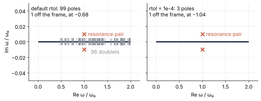
Reading the poles: physical ones and Froissart doublets. With Gaussian noise of σ = 10⁻⁶ on the samples the default rtol is out of reach, so AAA runs to its limit of 100 terms, warns, and returns 99 poles. Over 90 line the real axis inside [0, 2] in the left panel below, each with a zero nearby, a median 1.8 × 10⁻⁶ away: pairs that nearly cancel and fit the noise, called Froissart doublets. Their residues are at most 1.3 × 10⁻⁸, against 5.0 × 10⁻³ for the resonance pair. At the midpoints between samples the fit misses the true curve by 1.2 × 10⁻³, a thousand times the noise. clean_up, meant to remove doublets, keeps these: their residues are far above its clean_up_tol. With rtol=1e-4 AAA stops at four support points and finds the pair with Q = 50.0006. Each fit also has a real pole off the frame and outside the samples, at −0.68 and −1.04, with a residue of 1.4 × 10⁻⁴ and 2.5 × 10⁻⁴, too large for a doublet. It stands in for the mirror pair at −0.99995 ± 0.0100i, like the pole at −0.66856 of the noise-free fit with four support points, which the fifth turned into that pair. The rule: set rtol about 100 times the relative noise (10⁻⁶ here, so 10⁻⁴), distrust a pole whose residue is orders of magnitude below the others', and read a pole outside the samples as a sign of something there, not its position.

rng = np.random.default_rng(0)
y_noisy = power(x) + 1e-6 * rng.standard_normal(x.size)

with warnings.catch_warnings(record=True) as caught:   # print the warning, so both runs show the same text
    warnings.simplefilter("always")
    r_noisy = AAA(x, y_noisy)
for w in caught:
    print(f"{w.category.__name__}: {w.message}")

poles_n, res_n = r_noisy.poles(), r_noisy.residues()
doublet = np.abs(res_n) < 1e-4 * np.abs(res_n).max()
on_axis = (poles_n.imag == 0) & (poles_n.real > 0) & (poles_n.real < 2)
zeros_n = r_noisy.roots()
gap = np.array([np.min(np.abs(zeros_n - p)) for p in poles_n[doublet]])
mid = (x[:-1] + x[1:]) / 2
print(f"default rtol: {r_noisy.support_points.size} support points, {poles_n.size} poles, "
      f"{on_axis.sum()} of them on the real axis inside [0, 2]")
print(f"  {doublet.sum()} doublets, |residue| {np.abs(res_n[doublet]).min():.1e} to {np.abs(res_n[doublet]).max():.1e}, "
      f"median distance to the nearest zero {np.median(gap):.1e}")
pair = (np.abs(poles_n - a_pole) < 1e-3) | (np.abs(poles_n - a_pole.conjugate()) < 1e-3)
print(f"  resonance pair: |residue| {np.abs(res_n[pair]).round(5).tolist()}")
print(f"  max error at the sample midpoints against the true P: {np.max(np.abs(r_noisy(mid) - power(mid))):.1e}")

r_tol = AAA(x, y_noisy, rtol=1e-4)
poles_t = r_tol.poles()
up = poles_t[(poles_t.imag > 0) & (poles_t.real > 0)][0]
print(f"rtol=1e-4: {r_tol.support_points.size} support points, poles: {', '.join(fmt(p) for p in poles_t)}")
print(f"  Q from the upper pole: {abs(up) / (2 * up.imag):.4f}, max error against the true P {np.max(np.abs(r_tol(wf) - Pf)):.1e}")
for label, p_all, c_all in [("default rtol", poles_n, res_n), ("rtol=1e-4", poles_t, r_tol.residues())]:
    far = (p_all.real < -0.2) | (p_all.real > 2.2) | (np.abs(p_all.imag) > 0.05)   # off the frame below
    print(f"{label}: pole off the frame at {fmt(p_all[far][0])}, |residue| {abs(c_all[far][0]):.1e}")

RuntimeWarning: AAA failed to converge within 100 iterations.
default rtol: 100 support points, 99 poles, 94 of them on the real axis inside [0, 2]
  96 doublets, |residue| 1.5e-11 to 1.3e-08, median distance to the nearest zero 1.8e-06
  resonance pair: |residue| [0.005, 0.005]
  max error at the sample midpoints against the true P: 1.2e-03
rtol=1e-4: 4 support points, poles: -1.04152, +0.99995+0.01000i, +0.99995-0.01000i
  Q from the upper pole: 50.0006, max error against the true P 1.1e-05
default rtol: pole off the frame at -0.67514, |residue| 1.4e-04
rtol=1e-4: pole off the frame at -1.04152, |residue| 2.5e-04

Show code

Copy

fig, axes = plt.subplots(1, 2, sharey=True)
panels = [(axes[0], poles_n, doublet, "default rtol"), (axes[1], poles_t, np.zeros(poles_t.size, bool), "rtol = 1e-4")]
for ax, poles, spurious, label in panels:
    inside = (poles.real > -0.2) & (poles.real < 2.2) & (np.abs(poles.imag) < 0.05)
    near_pair = (np.abs(poles - a_pole) < 1e-3) | (np.abs(poles - a_pole.conjugate()) < 1e-3)
    ax.plot([0, 2], [0, 0], color=INK, lw=3, solid_capstyle="butt", zorder=1)
    ax.plot(poles[inside & spurious].real, poles[inside & spurious].imag, "|", color=MUTED, ms=16, mew=1, zorder=2)
    ax.plot(poles[near_pair].real, poles[near_pair].imag, "x", color=ACCENT, ms=8, mew=2, zorder=3)
    ax.text(1.08, a_pole.imag, "resonance pair", color=ACCENT, va="center")
    if spurious.any():
        ax.text(1.45, -0.009, f"{(inside & spurious).sum()} doublets", color=MUTED, ha="center", va="top")
    off = ", ".join(f"{p.real:.2f}".replace("-", "−") for p in poles[~inside])
    ax.text(0.02, 0.97, f"{label}: {poles.size} poles\n{(~inside).sum()} off the frame, at {off}",
            transform=ax.transAxes, va="top")
    ax.set(xlim=(-0.2, 2.2), ylim=(-0.05, 0.05), xlabel="Re ω / ω₀")
axes[0].set_ylabel("Im ω / ω₀")
fig.tight_layout()
plt.show()

See it in code

The whole job with the standard functions: AAA on the 2,000 noise-free samples, its poles and residues, and the resonance read off the pole a in the upper half plane near 1, with ω₀ = |a| and Q = |a| / (2 Im a). The same cell runs the polynomial over 29 degrees from 4 to 2048 for the comparison on the left.

Show code

Copy

r = AAA(x, power(x))
poles, res = r.poles(), r.residues()
a = poles[(poles.imag > 0) & (poles.real > 0)][0]
exact = np.array([a_pole, a_pole.conjugate(), -a_pole, -a_pole.conjugate()])
print(f"support points: {r.support_points.size}, max error {np.max(np.abs(r(wf) - Pf)):.1e}")
for p, c in sorted(zip(poles, res), key=lambda pc: (pc[0].real, pc[0].imag)):
    print(f"  pole {fmt(p):>21s}   |residue| {abs(c):.6f}")
print(f"largest distance to the exact poles: {max(np.min(np.abs(exact - p)) for p in poles):.1e}")
print(f"from the upper pole: ω₀ = {abs(a):.4f}, Q = {abs(a) / (2 * a.imag):.3f}")

degrees = np.unique(2 * np.round(np.geomspace(2, 1024, 30)).astype(int))
cheb_err = np.array([cheb_error(n)[0] for n in degrees])
with warnings.catch_warnings():
    warnings.simplefilter("ignore", RuntimeWarning)
    aaa_err = np.array([np.max(np.abs(AAA(x, power(x), max_terms=m)(wf) - Pf)) for m in range(1, 6)])
aaa_params = 2 * np.arange(1, 6) - 1
print(f"Chebyshev: {degrees.size} degrees, {degrees[-1] + 1} coefficients give {cheb_err[-1]:.1e}")
print(f"AAA: {aaa_params[-1]} numbers give {aaa_err[-1]:.1e}")

fig, (ax1, ax2) = plt.subplots(1, 2, figsize=(8, 3.4))
ax1.loglog(degrees + 1, cheb_err, "o-", color=SECOND, ms=4, lw=1.4)
ax1.loglog(aaa_params, aaa_err, "o-", color=ACCENT, ms=6)
ax1.axhline(np.finfo(float).eps, color=MUTED, lw=1, ls="--")
ax1.text(40, 1e-3, "Chebyshev", color=SECOND, va="top")
ax1.text(10, 1e-13, "AAA", color=ACCENT)
ax1.text(1.1, 3e-16, "ε", color=MUTED, va="bottom")
ax1.set(xlabel="number of parameters", ylabel="max error", ylim=(1e-16, 1e3))
ax2.plot([0, 2], [0, 0], color=INK, lw=3, solid_capstyle="butt")
ax2.plot(poles.real, poles.imag, "x", color=ACCENT, ms=8, mew=2)
ax2.annotate(f"{a.real:.5f} ± {a.imag:.4f}i, Q = {abs(a) / (2 * a.imag):.1f}", (a.real, a.imag),
             xytext=(-20, 12), textcoords="offset points", ha="center", color=ACCENT)
ax2.set(xlim=(-1.3, 2.3), ylim=(-0.03, 0.03), xlabel="Re ω / ω₀", ylabel="Im ω / ω₀")
fig.tight_layout()
plt.show()

support points: 5, max error 4.0e-15
  pole     -0.99995-0.01000i   |residue| 0.005000
  pole     -0.99995+0.01000i   |residue| 0.005000
  pole     +0.99995-0.01000i   |residue| 0.005000
  pole     +0.99995+0.01000i   |residue| 0.005000
largest distance to the exact poles: 2.6e-08
from the upper pole: ω₀ = 1.0000, Q = 50.000
Chebyshev: 29 degrees, 2049 coefficients give 1.4e-09
AAA: 9 numbers give 4.0e-15

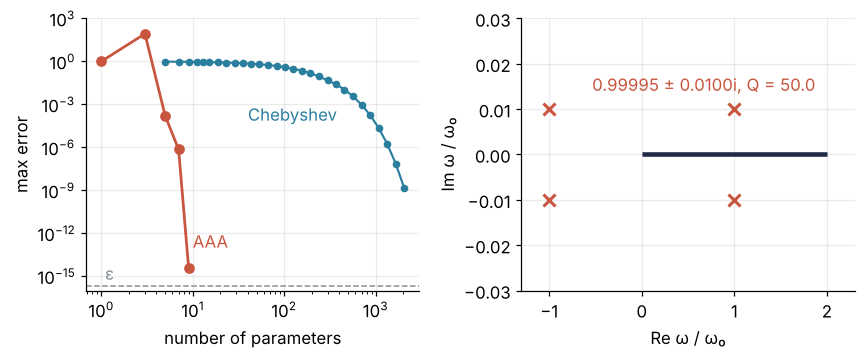
The poles of P are the roots of (1 − ω²)² + (ω/Q)², which are ±√(1 − 1/(4Q²)) ± i/(2Q) = ±0.99995 ± 0.0100i. AAA's four poles lie within 3 × 10⁻⁸ of them, and the fit returns ω₀ = 1.0000 and Q = 50.000 against the true 1 and 50. All four residues have magnitude 0.0050, the value of the Formalization, so there is no doublet and every pole is physical. On the left, nine numbers give fourteen digits, and the polynomial gets nine digits from 2,049.

Where it shows up

A pole near the real axis is the mathematical form of anything that rings, and wherever a response is measured or computed against frequency, a rational fit is the natural tool.

• Electrochemistry and materials. An impedance spectrum is fitted with an equivalent circuit, which is a rational function of frequency whose poles are the circuit's relaxation rates, one over each time constant. The dielectric function ε(ω) of a solid is fitted with a sum of Lorentz oscillators, one pole pair per resonance, which is the form that finite-difference time-domain (FDTD) simulations of light need.
• Electrical engineering. A Butterworth or Chebyshev filter is a rational transfer function by design. Vector fitting (Gustavsen and Semlyen, 1999) fits measured frequency responses of transformers, cables, and antennas with rational functions so that a circuit simulator can use them.
• Mechanical and control engineering. A finite-element model of a structure with a million unknowns has a transfer function whose few poles near the axis are its lightly damped modes. Model order reduction keeps those poles and drops the rest, and the reduced model runs in a controller.
• Physics. Quantum many-body codes compute response functions at imaginary frequencies, where they are smooth, and continue them to the real axis with Padé or AAA. The poles near the axis are the excitations, and their distance from the axis is the inverse lifetime, the 1/(2Q) of this tutorial.
• Mathematics. Rational approximation locates the zeros and poles of a function sampled on a curve in the complex plane. The "lightning" solvers of Gopal and Trefethen for Laplace problems are rational functions too, but they fix clusters of poles at the corners of a domain in advance, where the solution is singular, and fit only the coefficients by linear least squares.

In every case the pole is a resonance, a mode, or an excitation, and a rational fit hands you its position, and with it frequency and damping, as a number.

Further reading

• scipy.interpolate.AAA for rtol, clean_up, poles, and residues; mpmath.pade for the Padé route.
• Nakatsukasa, Sète, and Trefethen, "The AAA algorithm for rational approximation", SIAM J. Sci. Comput. 40, A1494 (2018).
• Trefethen, Approximation Theory and Approximation Practice, chapter 8 for the convergence rate on analytic functions and chapters 23 to 28 for rational approximation.
• Related tutorials on this site: The condition number: how many digits a linear solve can lose; Chebyshev collocation for eigenvalue problems: a neutron on a mirror, Chebyshev points at work; curve_fit from the ground up: the Michaelis-Menten constants of an enzyme, the route when the line shape is known and only its parameters are wanted. Planned: Chebyshev points: why crowding the samples toward the ends makes a polynomial converge.
• Download the notebook. It was executed with the library versions in the header.