Chebyshev collocation for eigenvalue problems: a neutron on a mirror (Python)

The problem: at which heights can a neutron bounce?

A slow neutron above a horizontal mirror falls, bounces, and falls again. Quantum mechanics allows it only certain energies, and experiments at the Institut Laue-Langevin see them. The lowest of these energy levels is 1.41 peV, and a classical neutron with that energy rises 13.7 μm above the mirror. Each level has a wavefunction ψ, and ψ² is the probability density of the neutron's height. Finding the levels is an eigenvalue problem for a differential operator, as finding squared frequencies was for a matrix in the normal modes tutorial. Chebyshev collocation turns the operator into a matrix, and scipy.linalg.eig does the rest.

Measure height in units of \(l_0 = (\hbar^2/2m^2g)^{1/3} = 5.868\) μm and energy in units of \(E_0 = (\hbar^2 m g^2/2)^{1/3} = 0.6018\) peV, with \(m\) the neutron mass. The stationary Schrödinger equation above the mirror is then

\[-\psi'' + x\,\psi = E\,\psi, \qquad \psi(0) = 0, \qquad \psi \to 0 \text{ for } x \to \infty ,\]

where \(x\) is the height, the term \(x\psi\) is gravity, and \(\psi(0) = 0\) is the mirror. The Airy function Ai is the solution of \(y'' = xy\) that decays for large \(x\), so the solution here that decays upward is Ai shifted by the energy, \(\mathrm{Ai}(x - E)\), and the mirror demands \(\mathrm{Ai}(-E) = 0\). The energies are the zeros of the Airy function with the sign flipped: 2.33811, 4.08795, 5.52056, and so on. A potential of your own will have no such answer, which is why this one makes a good test. A Fourier method, as in the KdV tutorial, would assume a periodic function, and a mirror is a wall.

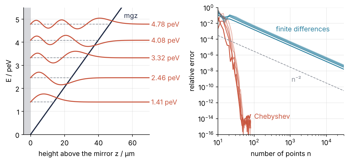
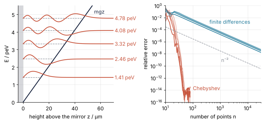
Left: the first five energy levels of a neutron above a mirror in peV against height in μm, each wavefunction drawn at its energy over the gravitational potential. Right: relative error against number of points, log-log; Chebyshev reaches 10⁻¹⁴ by 50 points, finite differences fall as n⁻².

The levels on the left come from one eig call on a 38 × 38 matrix. The right panel is a sweep over the number of points, against finite differences, and the six steps below build both.

Setup

The exact energies come from mpmath.airyaizero, which computes the Airy zeros to as many digits as you ask for, more than any result here can reach. The interval ends at L = 20, which is 117 μm; Step 5 checks whether that is far enough.

import numpy as np
import matplotlib.pyplot as plt
import mpmath
from scipy.linalg import eig, eigh_tridiagonal
from scipy.interpolate import BarycentricInterpolator
from scipy.integrate import trapezoid
from scipy.special import airy
from scipy.constants import hbar, m_n, e

g = 9.81                                                  # m/s^2
E0 = (hbar**2 * m_n * g**2 / 2) ** (1 / 3) / e * 1e12     # energy unit in peV
l0 = (hbar**2 / (2 * m_n**2 * g)) ** (1 / 3) * 1e6        # length unit in μm
a = np.array([-float(mpmath.airyaizero(k)) for k in range(1, 81)])   # exact levels, units of E0
L = 20.0                                                  # top of the interval, units of l0

plt.rcParams.update({                      # the look of every figure below
    "figure.figsize": (7, 3.6), "figure.dpi": 110,
    "axes.spines.top": False, "axes.spines.right": False,
    "axes.grid": True, "grid.alpha": 0.25,
    "font.size": 11, "lines.linewidth": 1.8,
})
INK, ACCENT, SECOND, MUTED = "#1f2a44", "#c8553d", "#2a7f9e", "#8a8f98"

print(f"energy unit {E0:.4f} peV, length unit {l0:.3f} μm, E1 = {a[0] * E0:.4f} peV at {a[0] * l0:.2f} μm")

energy unit 0.6018 peV, length unit 5.868 μm, E1 = 1.4070 peV at 13.72 μm

Step 1: Build the Chebyshev differentiation matrix

Collocation replaces the unknown function by its values at n points. Through n values passes exactly one polynomial of degree n − 1. Differentiate that polynomial and evaluate the derivative at the same n points, and each new value is a linear combination of the old ones: a matrix, D, the differentiation matrix.

The points are the Chebyshev points \(t_j = \cos\big(j\pi/(n-1)\big)\), \(j = 0, \dots, n-1\), which crowd toward both ends of [−1, 1]. On equally spaced points a polynomial of high degree swings wildly near the ends (more on that under interpolation and approximation). For the Chebyshev points the entries off the diagonal have a closed form,

\[D_{ij} = \frac{c_i}{c_j}\,\frac{(-1)^{i+j}}{t_i - t_j}, \qquad i \ne j ,\]

with \(c = 2\) at the two ends and 1 inside. The derivative of a constant is zero, so every row of D sums to zero, and that fixes the diagonal. The test function is Ai(2t). scipy.special.airy returns Ai, Ai′, Bi, and Bi′ in that order, so the exact derivative 2 Ai′(2t) comes with it.

def cheb_matrix(n):
    """Differentiation matrix on n Chebyshev points t, from t = 1 down to t = -1."""
    t = np.cos(np.pi * np.arange(n) / (n - 1))
    c = np.ones(n)
    c[[0, -1]] = 2
    sign = (-1.0) ** np.arange(n)
    dt = t[:, None] - t[None, :]
    np.fill_diagonal(dt, np.inf)                 # the diagonal comes out 0 here, set below
    D = np.outer(c * sign, sign / c) / dt
    D -= np.diag(D.sum(axis=1))                  # rows sum to zero
    return D, t

for n in [10, 20, 30, 40]:
    D, t = cheb_matrix(n)
    f, Ai_prime = airy(2 * t)[:2]
    df = 2 * Ai_prime                            # chain rule for the factor 2
    print(f"n = {n:2d}   max error of D @ f: {np.abs(D @ f - df).max():.1e}")

n = 10   max error of D @ f: 2.6e-04
n = 20   max error of D @ f: 5.1e-12
n = 30   max error of D @ f: 7.7e-14
n = 40   max error of D @ f: 8.9e-14

Doubling the points from 10 to 20 cut the error by a factor of about 5 × 10⁷, and at 30 points it reaches rounding. A method whose error falls as n⁻² gains a factor of 4 for the same doubling. An error that falls faster than any power of n is called spectral accuracy, and Step 6 measures the contrast on the neutron.

Step 2: Map to your interval and put in the walls

The neutron lives on [0, L]. The map x = L(1 − t)/2 takes t = 1 to the mirror at x = 0 and t = −1 to x = L. By the chain rule d/dx = −(2/L) d/dt: stretching the interval by L/2 flattens slopes by the same factor, and the sign flips because x runs the other way. The second derivative is the first applied twice.

Where ψ = 0, the first and last values are known zeros. Their columns multiply zero and drop out. Their rows, the equation at the walls, are replaced by the boundary conditions and drop out too, which leaves the inner block D2[1:-1, 1:-1]. To check both, solve −u″ = f for u = sin(πx/L) e^(−x/4), which vanishes at both walls, with one linear solve as in the resistor network tutorial:

def second_derivative(n, L):
    """Points x on [0, L] and the second derivative matrix, mirror first."""
    D, t = cheb_matrix(n)
    x = L * (1 - t) / 2
    Dx = -2 / L * D                              # chain rule: dt/dx = -2/L
    return x, Dx @ Dx

kappa = np.pi / L
for n in [10, 20, 30, 40]:
    x, D2 = second_derivative(n, L)
    u = np.sin(kappa * x) * np.exp(-x / 4)
    f = -np.exp(-x / 4) * ((1 / 16 - kappa**2) * np.sin(kappa * x) - kappa / 2 * np.cos(kappa * x))
    u_inner = np.linalg.solve(-D2[1:-1, 1:-1], f[1:-1])
    print(f"n = {n:2d}   max error of u: {np.abs(u_inner - u[1:-1]).max():.0e}")

n = 10   max error of u: 1e-06
n = 20   max error of u: 4e-16
n = 30   max error of u: 6e-16
n = 40   max error of u: 5e-15

Ten points get u right to 10⁻⁶, and from 20 on the error is rounding. That is the whole method for a boundary value problem.

Step 3: Solve the eigenvalue problem with eig

The left side of the equation, −ψ″ + xψ, becomes the matrix H = −D2 + diag(x) on the inner points. The potential sits on the diagonal because the term xψ at point j is x_j ψ_j and touches no other point. Before you pick an eigenvalue routine, ask whether H is symmetric, and if not, whether rescaling the unknowns could make it so, as it did for the masses in the normal modes tutorial. The cell prints two mirrored entries, the spacing of the points, and a product of three entries around a loop, which settles the rescaling question:

def hamiltonian(n, L, potential):
    x, D2 = second_derivative(n, L)
    return x, -D2[1:-1, 1:-1] + np.diag(potential(x[1:-1]))

x, H = hamiltonian(40, L, lambda x: x)
spacing = np.diff(x)
loop = H[0, 1] * H[1, 2] * H[2, 0] / (H[1, 0] * H[2, 1] * H[0, 2])
print(f"H[0,1] = {H[0, 1]:.0f}, H[1,0] = {H[1, 0]:.0f}")
print(f"spacing {spacing[0]:.2f} at the mirror, {spacing.max():.2f} in the middle")
print(f"loop ratio H01 H12 H20 / (H10 H21 H02) = {loop:.3f}")

H[0,1] = -371, H[1,0] = -173
spacing 0.03 at the mirror, 0.81 in the middle
loop ratio H01 H12 H20 / (H10 H21 H02) = 0.851

H is not symmetric: H[0,1] is −371 and H[1,0] is −173. Entry (i, j) is the weight the value at x_j gets in the second derivative at x_i, and with points 0.03 apart at the mirror and 0.81 in the middle, what one point gives its neighbor is not what it gets back.

Rescaling each unknown by a factor \(s_i\), as that tutorial did in its Step 5 with \(s_i = \sqrt{m_i}\), multiplies entry (i, j) by \(s_i/s_j\). Around a loop of three points the factors cancel, \((s_0/s_1)(s_1/s_2)(s_2/s_0) = 1\), so the loop ratio is the same after any rescaling, and 1 for a symmetric matrix. Here it is 0.851: no rescaling of the unknowns makes H symmetric, and the routine is scipy.linalg.eig:

w, U = eig(H)
print("first three as returned:", np.round(w[:3], 0))

order = np.argsort(w.real)                       # one index for values and vectors
lam, U = w[order].real, U[:, order].real
for j in range(5):
    print(f"level {j + 1}: {lam[j]:.10f}  exact {a[j]:.10f}  error {lam[j] - a[j]:+.0e}"
          f"  = {lam[j] * E0:.3f} peV")
print(f"largest imaginary part: {np.abs(w.imag).max():.0e}")

first three as returned: [1099.+0.j 1119.+0.j  193.+0.j]
level 1: 2.3381074105  exact 2.3381074105  error -4e-13  = 1.407 peV
level 2: 4.0879494441  exact 4.0879494441  error -8e-12  = 2.460 peV
level 3: 5.5205598281  exact 5.5205598281  error -4e-11  = 3.322 peV
level 4: 6.7867080900  exact 6.7867080901  error -1e-10  = 4.084 peV
level 5: 7.9441335869  exact 7.9441335871  error -2e-10  = 4.781 peV
largest imaginary part: 0e+00

eig returns complex numbers in no particular order, so one np.argsort on the real parts sorts the values and, applied to the columns, the eigenvectors. Forty points give the five lowest energies to ten digits, 1.407 to 4.781 peV. The imaginary parts are all 0, so .real loses nothing. If yours are not, check that your potential array is real, and treat a complex value like any eigenvalue that fails a rerun; Step 5 shows how.

Step 4: Turn the eigenvectors into wavefunctions

An eigenvector holds ψ at the 38 inner points, scaled so that the squares of these 38 numbers sum to 1. That is not the physical normalization ∫ψ² dx = 1, and 38 points are too few to draw. Put the zeros back at both walls, and BarycentricInterpolator evaluates the polynomial through the 40 values, the same polynomial D differentiates, on as fine a grid as you like. trapezoid normalizes it, and the sign is chosen so that ψ rises from the mirror. The exact wavefunctions, \(\mathrm{Ai}(x - a_k)\) from scipy.special.airy, get the same treatment:

def normalized(values, z):
    psi = values / np.sqrt(trapezoid(values**2, z))
    return psi if psi[1] > 0 else -psi              # rise from the mirror

z = np.linspace(0, L, 2001)
psi = np.array([normalized(BarycentricInterpolator(x, np.r_[0, U[:, j], 0])(z), z)
                for j in range(5)])
for j in range(5):
    exact = normalized(airy(z - a[j])[0], z)
    print(f"level {j + 1}: max difference to Ai {np.abs(psi[j] - exact).max():.0e}")

z_um, E_peV = l0 * z, E0 * lam                      # physical units: μm and peV

level 1: max difference to Ai 6e-12
level 2: max difference to Ai 3e-10
level 3: max difference to Ai 2e-09
level 4: max difference to Ai 1e-08
level 5: max difference to Ai 6e-08

The wavefunctions are less accurate than the energies, from 6 × 10⁻¹² for level 1 to 6 × 10⁻⁸ for level 5, and still far beyond anything a plot can show. The last line converts to micrometers and peV for the figure in Step 6.

Step 5: Tell which eigenvalues to trust

Forty points gave 38 eigenvalues. Here is how many deserve the name:

def levels(n, L, potential=lambda x: x):
    """Step 3 in one call: sorted eigenvalues, eigenvectors, and points."""
    x, H = hamiltonian(n, L, potential)
    w, U = eig(H)
    order = np.argsort(w.real)
    return w[order].real, U[:, order].real, x

for j in [1, 5, 10, 11, 13, 20, 38]:
    print(f"level {j:2d}: {lam[j - 1]:10.6f}  exact {a[j - 1]:9.6f}  error {lam[j - 1] - a[j - 1]:+.0e}")

level  1:   2.338107  exact  2.338107  error -4e-13
level  5:   7.944134  exact  7.944134  error -2e-10
level 10:  12.828776  exact 12.828777  error -6e-07
level 11:  13.691487  exact 13.691489  error -2e-06
level 13:  15.340723  exact 15.340755  error -3e-05
level 20:  20.744468  exact 20.537333  error +2e-01
level 38: 1118.801218  exact 31.630556  error +1e+03

Ten levels are within 10⁻⁶ of the exact values, the next ones drift off slowly, and the top of the list is nonsense: 1119 where the 38th Airy zero is 31.6. Two things cause this: the wall at L pushes up every level whose wavefunction still reaches it, and a polynomial of degree 39 can follow only so many oscillations. More points and a longer interval show both:

runs = [(40, 20.0), (80, 20.0), (80, 30.0)]
k = np.arange(1, 41)
fig, ax = plt.subplots()
for (n, L_run), alpha in zip(runs, [0.45, 0.7, 1.0]):         # all Chebyshev: one color, darker reaches further
    w_run = levels(n, L_run)[0][:40]
    err = np.maximum(np.abs(w_run / a[:len(w_run)] - 1), 1e-16)
    ax.semilogy(k[:len(w_run)], err, "o-", color=ACCENT, alpha=alpha, ms=4, lw=1.2)
    ax.text(k[len(w_run) - 1] + 0.9, err[-1], f"n = {n}, L = {L_run:.0f}",
            color=ACCENT, alpha=0.5 + alpha / 2, va="center")   # labels stay legible
ax.semilogy(k, 1e-6 / a[:40], color=MUTED, ls="--", lw=1)
ax.text(31, 1e-8, "absolute error 10⁻⁶", color=MUTED, va="top")
ax.set(xlabel="level index k", ylabel="relative error of level k", xlim=(0, 49), ylim=(3e-17, 1e2))
plt.show()

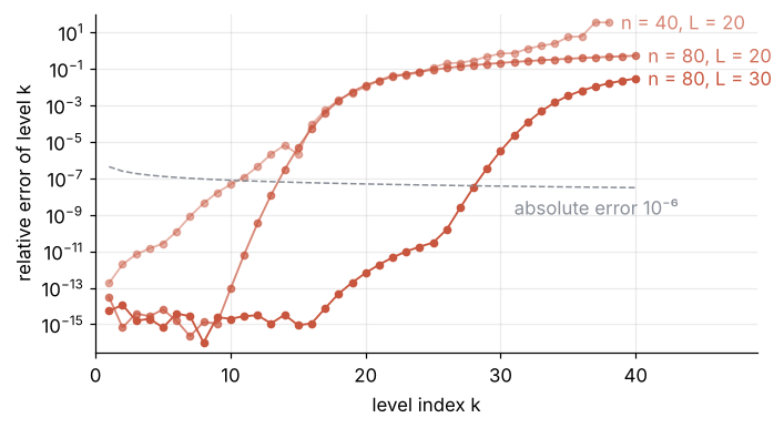
Relative error of each energy level against the level index k, log scale, for three runs. 40 points and L = 20: correct up to k = 10. 80 points, L = 20: up to 13. 80 points, L = 30: up to 28. A dashed line marks an absolute error of 10⁻⁶.

Twice the points buy only three more levels, because the wall at L = 20 now limits; at L = 30 the count is 28. The dashed line is an absolute error of 10⁻⁶ divided by a_k. Without an exact answer, rerun: pair the k-th eigenvalues of both runs and count up to the first pair that differs by more than your accuracy, here 10⁻⁶.

When L only truncates a half-infinite domain, as under open sky, rerun at 1.5 n and 1.5 L together: the longer interval tests the wall, the extra points the resolution. Going from (n, L) = (40, 20) to (60, 30) raises the degree from 39 to 59 at nearly the same average spacing, and since the added length holds only decaying tails, the extra degree goes to the oscillations of the low levels: level 11 moves from 2 × 10⁻⁶ to 7 × 10⁻¹⁰ off, and its pair fails.

When L is a real wall, rerun at 1.5 n only, because a different L is a different problem. Read the run (80, 20) as a neutron under a ceiling at height 20: its lowest 39 levels agree with the rerun at 120 points, and a 240-point run confirms all 39. The joint rerun moves the ceiling, so only 13 agree.

def agreeing(w1, w2, tol=1e-6):
    """How many eigenvalues, from the lowest up, agree between two sorted runs."""
    m = min(len(w1), len(w2))
    off = np.abs(w1[:m] - w2[:m]) > tol
    return int(np.argmax(off)) if off.any() else m

print("  n   L   correct, no ceiling   joint rerun   n-only rerun")
for n, L_run in runs:
    w1 = levels(n, L_run)[0]
    w_joint = levels(int(1.5 * n), 1.5 * L_run)[0]
    w_n = levels(int(1.5 * n), L_run)[0]
    print(f"{n:3d} {L_run:3.0f}   {agreeing(w1, a):19d}   {agreeing(w1, w_joint):11d}"
          f"   {agreeing(w1, w_n):12d}")

w60 = levels(60, 30.0)[0]
print(f"level 11: error {lam[10] - a[10]:+.0e} at (40, 20), {w60[10] - a[10]:+.0e} at (60, 30)")
w_ceiling = levels(80, 20.0)[0]
print(f"ceiling at 20, n = 80: {agreeing(w_ceiling, levels(240, 20.0)[0])} levels agree with 240 points")

  n   L   correct, no ceiling   joint rerun   n-only rerun
 40  20                    10            10             10
 80  20                    13            13             39
 80  30                    28            28             34
level 11: error -2e-06 at (40, 20), -7e-10 at (60, 30)
ceiling at 20, n = 80: 39 levels agree with 240 points

The joint column matches the first in every row. At (80, 30) the n-only rerun also passes levels 29 to 34, converged under a ceiling at height 30 but not under open sky. At (40, 20) both say 10: resolution is the limit.

Step 6: Compare with finite differences and draw the levels

The three-point formula of the leapfrog tutorial and the findiff tutorial, (ψ_{j−1} − 2ψ_j + ψ_{j+1})/h² on n equally spaced points, gives a tridiagonal matrix. It is symmetric, because equal spacing gives the same weight 1/h² both ways, unlike Step 3's H. So eigh_tridiagonal with select="i" returns only the five lowest levels and handles 30,000 points in a fraction of a second. The cell sweeps both and draws the figure from the top, each color fading from level 1 to level 5:

def fd_levels(n, L):
    """Five lowest levels with the three-point formula on n equally spaced points."""
    x_fd = np.linspace(0, L, n)
    h = x_fd[1] - x_fd[0]
    diag = 2 / h**2 + x_fd[1:-1]
    return eigh_tridiagonal(diag, np.full(n - 3, -1 / h**2), select="i", select_range=(0, 4))[0]

n_cheb = np.arange(10, 81, 2)
n_fd = np.unique(np.geomspace(10, 30000, 22).round().astype(int))
err_cheb = np.array([np.abs(levels(n, L)[0][:5] / a[:5] - 1) for n in n_cheb])
err_fd = np.array([np.abs(fd_levels(n, L) / a[:5] - 1) for n in n_fd])

fig, (ax1, ax2) = plt.subplots(1, 2, figsize=(8, 3.8))
z_top = 70
ax1.axvspan(-4, 0, color=MUTED, alpha=0.35, lw=0)
ax1.plot([0, z_top], [0, E0 * z_top / l0], color=INK)
scale = 0.35 / np.abs(psi).max()
for j in range(5):
    turn = l0 * a[j]
    ax1.plot([0, turn], [E0 * a[j]] * 2, color=MUTED, ls="--", lw=1)
    ax1.plot(z_um, E_peV[j] + scale * psi[j], color=ACCENT, lw=1.6)
    ax1.text(z_top + 1, E0 * a[j], f"{E0 * a[j]:.2f} peV", va="center", color=ACCENT)
ax1.text(55, 5.05, "mgz", color=INK)
ax1.set(xlabel="height above the mirror z / μm", ylabel="E / peV", xlim=(-4, z_top), ylim=(0, 5.5))

for j in range(5):
    alpha = 1.0 - 0.15 * j
    ax2.loglog(n_cheb, np.maximum(err_cheb[:, j], 1e-16), color=ACCENT, alpha=alpha, lw=1.4)
    ax2.loglog(n_fd, err_fd[:, j], color=SECOND, alpha=alpha, lw=1.4)
ax2.loglog(n_fd, 3e-4 * (n_fd / 10.0) ** -2, color=MUTED, ls="--", lw=1)
ax2.text(100, 1e-14, "Chebyshev", color=ACCENT)
ax2.text(400, 1e-3, "finite differences", color=SECOND)
ax2.text(2000, 3e-9, "n⁻²", color=MUTED, ha="right", va="top")
ax2.set(xlabel="number of points n", ylabel="relative error", xlim=(10, 3e4), ylim=(1e-16, 1))
fig.tight_layout()
plt.show()

fd40 = np.abs(fd_levels(40, L) / a[:5] - 1)
print(f"n = 40, Chebyshev:          level 1 off by {err_cheb[n_cheb == 40][0, 0]:.0e}, level 5 by {err_cheb[n_cheb == 40][0, 4]:.0e}")
print(f"n = 40, finite differences: level 1 off by {fd40[0]:.0e}, level 5 by {fd40[4]:.0e}")
print(f"level 1 below 1e-6 from n = {n_cheb[np.argmax(err_cheb[:, 0] < 1e-6)]} (Chebyshev), "
      f"n = {n_fd[np.argmax(err_fd[:, 0] < 1e-6)]} (finite differences)")

Left: energy in peV against height in μm, with the rising gravitational potential and the first five wavefunctions at their energies, 1.41 to 4.78 peV. Right: relative error of levels 1 to 5 against number of points, log-log; Chebyshev falls to 10⁻¹⁴ by 50 points, finite differences as n⁻².

n = 40, Chebyshev:          level 1 off by 2e-13, level 5 by 3e-11
n = 40, finite differences: level 1 off by 1e-02, level 5 by 4e-02
level 1 below 1e-6 from n = 22 (Chebyshev), n = 4459 (finite differences)

At 40 points finite differences are off by 1 % on level 1 and 4 % on level 5, where Chebyshev is off by 2 × 10⁻¹³ and 3 × 10⁻¹¹. They gain a factor of 100 for every factor of 10 in n, the n⁻² of a three-point formula, and need 4,459 points of the sweep to bring level 1 below a relative error of 10⁻⁶, which Chebyshev does with 22. Chebyshev reaches rounding at about 50 points.

Pitfalls

Using eigh on the collocation matrix. There is no warning, and the ground state comes out wrong:

from scipy.linalg import eigh
print("eigh:", np.round(eigh(H, eigvals_only=True)[:3], 2), "  exact:", np.round(a[:3], 3))

eigh: [3.4  4.86 6.15]   exact: [2.338 4.088 5.521]

eigh reads one triangle of H and mirrors it, so it solves a different, symmetric matrix and returns 3.40 for a ground state of 2.338. Use eig, and before you try to symmetrize a matrix of your own, compute Step 3's loop ratio.

An interval too short. The levels that reach the wall come out too high, never too low, and more points do not help. At L = 10 the errors of levels 1 to 5 are these, at 40 and at 80 points:

Show code

for n in [40, 80]:
    errs = levels(n, 10.0)[0][:5] - a[:5]
    print(f"n = {n}, L = 10:  " + "  ".join(f"{d:+.0e}" for d in errs))

n = 40, L = 10:  +1e-13  +1e-09  +7e-07  +9e-05  +3e-03
n = 80, L = 10:  +3e-13  +1e-09  +7e-07  +9e-05  +3e-03

Level 1 sits at rounding, and levels 2 to 5 do not move by a digit when the points double. The wall squeezes every wavefunction that reaches past its turning point, which raises its energy. The sign and the frozen digits identify the wall without an exact answer. Raise L together with n.

Sorting the eigenvalues but not the eigenvectors. The "ground state" has nodes, or jumps from point to point, because it belongs to the eigenvalue 1099. np.sort(w) reorders only the values. Take one index from np.argsort(w.real) and apply it to both, as Step 3 does.

Variations

A ceiling above the neutron. qBounce puts an absorber above the mirror, and in the simplest model it is a second wall. Set L to the slit height in units of l₀ and watch the upper levels rise above the Airy values; trust them by Step 5's real-wall rerun.
The harmonic oscillator. Map to [−L, L] instead, with x = Lt and Dx = D / L, and use the potential x². The eigenvalues are 2k + 1, the standard check of any eigenvalue code.
A wall value other than zero. In Step 2's boundary value problem, the columns you dropped no longer multiply zero: move the wall values times the first and last columns of D2, inner rows only, to the right-hand side.
Time dependence. The same D2 as the right-hand side of solve_ivp, the method of lines, gives the heat equation or the time-dependent Schrödinger equation between walls, as the FFT derivative did in the KdV tutorial. The largest eigenvalue, Step 3's 1119, grows like n⁴, so the largest stable explicit step shrinks like n⁻⁴; the stiffness tutorial says what to do about that.

Cheat sheet

t = np.cos(np.pi * np.arange(n) / (n - 1))                   # n Chebyshev points, t[0] = 1
c, sign = np.r_[2, np.ones(n - 2), 2], (-1.0) ** np.arange(n)
dt = np.subtract.outer(t, t); np.fill_diagonal(dt, np.inf)   # keeps the diagonal 0 for now
D = np.outer(c * sign, sign / c) / dt                        # D_ij = (c_i/c_j) (-1)^(i+j) / (t_i - t_j)
D -= np.diag(D.sum(axis=1))                                  # rows sum to 0: d/dt of a constant
x, Dx = L * (1 - t) / 2, -2 / L * D                          # [0, L], mirror at t = 1
H = -(Dx @ Dx)[1:-1, 1:-1] + np.diag(V(x[1:-1]))             # psi = 0 at both walls: drop them
w, U = scipy.linalg.eig(H); order = np.argsort(w.real)       # not symmetric: eig, never eigh
w, U = w[order].real, U[:, order].real                       # one index for values and vectors
# trust what agrees to your tolerance with (1.5 n, 1.5 L) if L truncates, with (1.5 n, L) if L is a wall