scikit-fem from the ground up: the sag of a membrane under pressure (Python)

The problem: how far does a clamped membrane sag?

Stretch a square membrane of side L = 0.1 m over a frame with a tension of T = 100 N/m, clamp all four edges, and press on it from one side with p = 200 Pa. It sags most at the center, by 1.47 mm. That number comes from a series that exists for the square and for little else. For an L-shaped frame, or any outline a real part has, you need finite elements, and scikit-fem is a Python package that assembles finite element matrices from the weak form you write down in a few lines of Python.

The deflection \(w\) obeys

\[-T\,\nabla^2 w = p, \qquad w = 0 \text{ on the edges},\]

where \(\nabla^2 w = \partial^2 w/\partial x^2 + \partial^2 w/\partial y^2\), the Laplacian, adds up the curvatures in the two directions: the membrane settles where tension times curvature balances the pressure. Substituting \(x = L\xi\) and \(w = (pL^2/T)\,u\) turns every square membrane into the same problem, \(-\nabla^2 u = 1\) on the unit square with \(u = 0\) on the edges. Its double Fourier series puts the center at \(u = 0.07367\), so the sag is \(0.0737\,pL^2/T\). Under other names the same equation gives the stress function of a twisted square bar and the temperature of a uniformly heated plate with cold edges.

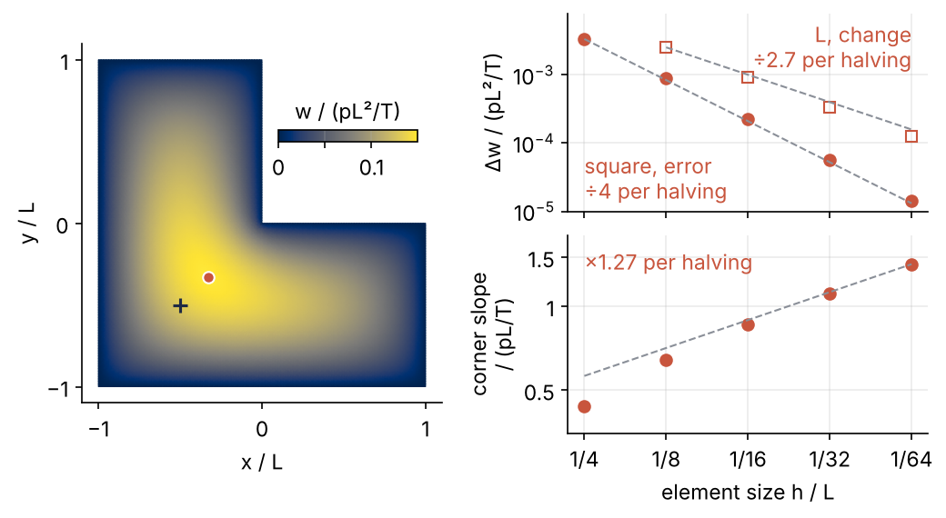
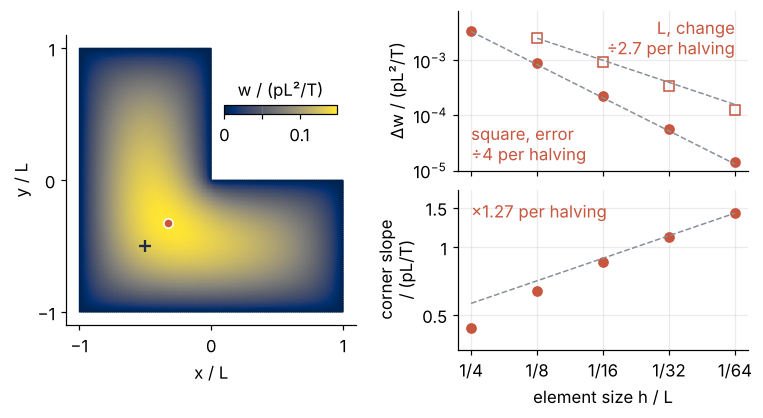
Left: color map of the deflection of an L-shaped membrane over x/L and y/L; a dot marks the peak, off the elbow center (plus) toward the inner corner. Right, against element size: the errors fall by four and by about 2.7 per halving, while the slope at the inner corner keeps rising.

This is where we end up: the L-shaped membrane, which has no formula, solved on a mesh of 24,576 triangles, and beside it what happens to the answers as the elements are halved. On the square the error falls by four per halving, on the L more slowly, and the slope at the inner corner never settles. Step 6 draws it.

Setup

Install the package with pip install scikit-fem; it imports as skfem.

import numpy as np
import matplotlib.pyplot as plt
from skfem import MeshTri, Basis, ElementTriP1, BilinearForm, LinearForm, asm, condense, solve
from skfem.helpers import dot, grad

L, T, p = 0.1, 100.0, 200.0         # m, N/m, Pa
SCALE = p * L**2 / T                # m; the deflection w is SCALE times the scaled u
W_EXACT = 0.0736713532              # u at the center of the unit square, from the double Fourier series

plt.rcParams.update({
    "figure.figsize": (7, 3.6), "figure.dpi": 110,
    "axes.spines.top": False, "axes.spines.right": False,
    "axes.grid": True, "grid.alpha": 0.25,
    "font.size": 11, "lines.linewidth": 1.8,
})
INK, ACCENT, SECOND, MUTED = "#1f2a44", "#c8553d", "#2a7f9e", "#8a8f98"

print(f"sag scale pL^2/T = {SCALE:.2f} m, series sag at the center = {W_EXACT * SCALE * 1e3:.2f} mm")

sag scale pL^2/T = 0.02 m, series sag at the center = 1.47 mm

Step 1: Cover the square with triangles

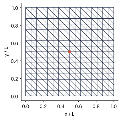
MeshTri() is the unit square cut along one diagonal into two triangles. .refined(4) splits every triangle into four, four times over, which leaves triangles with legs of h = 1/16:

mesh = MeshTri().refined(4)
print(mesh)
print("p:", mesh.p.shape, "  t:", mesh.t.shape)
print("first triangle, node indices:", mesh.t[:, 0])
print("its corners (x in the first row, y in the second):")
print(mesh.p[:, mesh.t[:, 0]])

<skfem MeshTri1 object>
  Number of elements: 512
  Number of vertices: 289
  Number of nodes: 289
p: (2, 289)   t: (3, 512)
first triangle, node indices: [ 0 81 82]
its corners (x in the first row, y in the second):
[[0.     0.0625 0.    ]
 [0.     0.     0.0625]]

512 triangles on 289 nodes, and the whole mesh is two NumPy arrays: mesh.p holds the coordinates of the nodes, one column per node, and mesh.t the three node numbers of each triangle, one column per triangle. Nothing ties a triangle to its neighbors except shared node numbers, which is why a mesh can follow any outline where the grid of py-pde from the ground up: the heat equation on a square plate is stuck with rectangles. A small helper finds the node nearest a point; the center of the square is a node, so the sag can be read there without interpolating.

def node_at(mesh, x, y):
    return np.argmin(np.hypot(mesh.p[0] - x, mesh.p[1] - y))

center = node_at(mesh, 0.5, 0.5)
print("center node:", center, "at", mesh.p[:, center])

center node: 6 at [0.5 0.5]

Show code

fig, ax = plt.subplots(figsize=(4, 4))
ax.triplot(mesh.p[0], mesh.p[1], mesh.t.T, color=INK, lw=0.8)
ax.plot(*mesh.p[:, center], "o", color=ACCENT, ms=6)
ax.set(xlabel="x / L", ylabel="y / L", aspect="equal")
ax.grid(False)
plt.show()

The unit square covered by 512 triangles of leg 1/16, x/L and y/L from 0 to 1, with the center node at (0.5, 0.5) marked.

Step 2: Write the weak form as two Python functions

The answer will be built from functions that are linear on each triangle. Their second derivatives are zero inside a triangle and undefined across its edges, so \(-\nabla^2 u\) cannot even be evaluated for them. The weak form gets around this by moving one derivative onto a second function. Multiply the equation by a test function \(v\) that vanishes on the clamped edges and integrate over the square, with \(f\) the scaled load, 1 everywhere for now:

\[\int (-\nabla^2 u)\, v \, dA = \int f\, v\, dA .\]

The divergence theorem applied to \(v\nabla u\), the two-dimensional version of integration by parts, rewrites the left side:

\[\int (-\nabla^2 u)\, v\, dA = \int \nabla u \cdot \nabla v\, dA - \oint v\, \frac{\partial u}{\partial n}\, ds ,\]

with \(\partial u/\partial n\) the slope across the edge. The edge integral is zero, because \(v\) is zero there. What remains is the weak form,

\[\int \nabla u\cdot\nabla v\, dA = \int f\, v\, dA \quad \text{for every } v,\]

and it needs only first derivatives. In scikit-fem each side is a Python function of the integrand, decorated to say which kind it is:

@BilinearForm
def stiffness(u, v, w):
    return dot(grad(u), grad(v))

@LinearForm
def load(v, w):
    return 1.0 * v

@LinearForm
def ramp(v, w):
    return w.x[0] * v

u is the trial function, the unknown, and v the test function; dot and grad from skfem.helpers act on all integration points at once. The third argument w, unrelated to the deflection \(w\), carries everything else; w.x holds the x and y coordinates of the points where scikit-fem evaluates the integrals. Any load \(f(x, y)\) is therefore a NumPy expression in w.x[0] and w.x[1], times v. ramp is a pressure that rises linearly from zero at one edge to full at the other, as on a panel in the wall of a water tank.

Step 3: Assemble one equation per node and solve

Basis(mesh, ElementTriP1()) gives one hat function \(\varphi_j\) per node: 1 at its node, 0 at every other node, linear on each triangle. The answer is written as \(u = \sum_j U_j \varphi_j\), so \(U_j\) is the deflection at node \(j\). Taking \(v = \varphi_i\) in the weak form gives one equation per node,

\[\sum_j A_{ij} U_j = f_i, \qquad A_{ij} = \int \nabla\varphi_i\cdot\nabla\varphi_j\, dA, \qquad f_i = \int f\,\varphi_i\, dA .\]

Each unknown \(U_j\) is a degree of freedom, a DOF. asm does the integrals:

basis = Basis(mesh, ElementTriP1())
print(basis)
A = asm(stiffness, basis)
f = asm(load, basis)
print(f"A: {A.shape}, {A.nnz} of {A.shape[0]**2} entries nonzero")
print("integration points as w.x sees them:", basis.global_coordinates().value.shape)

<skfem CellBasis(MeshTri1, ElementTriP1) object>
  Number of elements: 512
  Number of DOFs: 289
  Size: 110592 B
A: (289, 289), 1377 of 83521 entries nonzero
integration points as w.x sees them: (2, 512, 3)

289 DOFs, one per node. Only 1,377 of the 83,521 entries of A are nonzero, because \(\varphi_i\) and \(\varphi_j\) overlap only when nodes \(i\) and \(j\) share a triangle. The two ends of a diagonal share two triangles, yet in both one hat function rises along x and the other along y, so \(\nabla\varphi_i\cdot\nabla\varphi_j = 0\) and asm stores nothing. Poisson's equation with scipy.sparse: two plates in a grounded box builds such a matrix by hand. The last line is the shape of w.x: x and y, for 512 triangles, at three points each.

mesh.boundary_nodes() lists the clamped nodes. Their rows belong to test functions the weak form excludes, since \(v\) vanishes there; condense drops those rows and the matching columns, and solve puts the zeros back after solving for the rest:

boundary = mesh.boundary_nodes()
u = solve(*condense(A, f, D=boundary))
print(f"clamped nodes: {len(boundary)}")
print(f"center: u = {u[center]:.6f}   series {W_EXACT:.6f}   error {100 * (u[center] / W_EXACT - 1):+.2f} %")
print(f"for the 0.1 m membrane: w = {u[center] * SCALE * 1e3:.2f} mm")

clamped nodes: 64
center: u = 0.073446   series 0.073671   error -0.31 %
for the 0.1 m membrane: w = 1.47 mm

The finite element answer is 0.3 % low, 1.47 mm for the real membrane, because a membrane that bends only along element edges is stiffer than the real one. The ramp needs a new right-hand side and nothing else:

u_ramp = solve(*condense(A, asm(ramp, basis), D=boundary))
print(f"ramp load: center u = {u_ramp[center]:.6f}, {u_ramp[center] / u[center]:.4f} of the uniform load")

ramp load: center u = 0.036723, 0.5000 of the uniform load

Exactly half. A half turn about the center maps this mesh onto itself and the point \((x, y)\) onto \((1 - x, 1 - y)\). The ramp depends on \(x\) only, so it becomes the load \(1 - x\) with the same sag at the center, and the two loads add up to the uniform one.

Step 4: Halve the elements and watch the error fall by four

Wrap Step 3 in a function and solve on five meshes, from h = 1/4 to h = 1/64:

def solve_membrane(mesh):
    basis = Basis(mesh, ElementTriP1())
    A = asm(stiffness, basis)
    f = asm(load, basis)
    return basis, solve(*condense(A, f, D=mesh.boundary_nodes()))

levels = [2, 3, 4, 5, 6]
h = 1.0 / 2.0**np.array(levels)
err_square = []
print("   h    triangles   u(center)     error   ratio")
for n in levels:
    mesh_n = MeshTri().refined(n)
    _, u_n = solve_membrane(mesh_n)
    err_square.append(W_EXACT - u_n[node_at(mesh_n, 0.5, 0.5)])
    ratio = f"{err_square[-2] / err_square[-1]:6.2f}" if n > levels[0] else ""
    print(f"1/{2**n:<3d} {mesh_n.t.shape[1]:9d}   {u_n[node_at(mesh_n, 0.5, 0.5)]:.6f}  {err_square[-1]:.2e}  {ratio}")
err_square = np.array(err_square)

   h    triangles   u(center)     error   ratio
1/4          32   0.070313  3.36e-03  
1/8         128   0.072783  8.89e-04    3.78
1/16        512   0.073446  2.26e-04    3.94
1/32       2048   0.073615  5.66e-05    3.98
1/64       8192   0.073657  1.42e-05    4.00

Each halving divides the error by 3.78, 3.94, 3.98, 4.00: it falls as h², which is what linear elements promise when the exact solution is smooth. The slopes converge one power slower, as h in the mean-square sense, because a function that is linear on each triangle follows the slope of a curve only to first order. Never report a finite element number from one mesh. Halve the elements and check that the change falls by the factor the method promises.

Step 5: Swap the square for an L-shaped membrane

MeshTri.init_lshaped() is three unit squares around the origin, with the quadrant x > 0, y > 0 missing, and solve_membrane takes it unchanged. With no series to compare with, the table shows the deflection at (−0.5, −0.5), the elbow center and a node on every mesh, its change per halving and the ratio of successive changes, then the largest slope \(|\nabla u|\) in the triangles touching the inner corner and its growth. basis.interpolate(u).grad gives the gradient at each triangle's three integration points, equal for linear elements, so [:, :, 0] keeps the first.

u_elbow, slope_corner = [], []
print("   h    u(elbow)    change   ratio   corner slope   growth")
for n in levels:
    mesh_L = MeshTri.init_lshaped().refined(n)
    basis_L, u_L = solve_membrane(mesh_L)
    u_elbow.append(u_L[node_at(mesh_L, -0.5, -0.5)])
    slope = np.linalg.norm(basis_L.interpolate(u_L).grad[:, :, 0], axis=0)
    at_corner = np.any(np.hypot(*mesh_L.p[:, mesh_L.t]) == 0, axis=0)   # triangles with a node at the origin
    slope_corner.append(slope[at_corner].max())
    line = f"1/{2**n:<3d}  {u_elbow[-1]:.5f}"
    if n > levels[0]:
        line += f"  {u_elbow[-1] - u_elbow[-2]:.2e}"
        line += f"  {(u_elbow[-2] - u_elbow[-3]) / (u_elbow[-1] - u_elbow[-2]):5.2f}" if n > levels[1] else "       "
        line += f"  {slope_corner[-1]:11.3f}  {slope_corner[-1] / slope_corner[-2]:7.2f}"
    else:
        line += f"  {'':8s}  {'':5s}  {slope_corner[-1]:11.3f}"
    print(line)
change_L = np.diff(u_elbow)
slope_corner = np.array(slope_corner)

   h    u(elbow)    change   ratio   corner slope   growth
1/4    0.12705                         0.436
1/8    0.12959  2.53e-03               0.639     1.47
1/16   0.13051  9.20e-04   2.76        0.858     1.34
1/32   0.13085  3.38e-04   2.72        1.110     1.29
1/64   0.13097  1.27e-04   2.67        1.416     1.27

The deflection at the elbow center settles near 0.131, but the changes shrink by 2.76, 2.72, 2.67 per halving instead of four. The corner slope does not converge at all: it grows by 1.47, 1.34, 1.29, 1.27 per halving.

Both columns come from one fact. Near a corner of 270° the exact solution goes like \(r^{2/3}\), with \(r\) the distance from the corner. Its slope goes like \(r^{-1/3}\), infinite at \(r = 0\), and the corner triangles sit at \(r \approx h\), so each halving finds a slope \(2^{1/3} = 1.26\) times larger. A triangle there has one constant slope and misses the true one by about the slope itself, \(h^{-1/3}\); squared and integrated over the corner triangles' area, of order \(h^2\), that gives \(h^{4/3}\), so the mean-square slope error goes as \(h^{2/3}\) instead of h. The value error again gets twice the power, \(h^{4/3}\): each halving should divide the change by \(2^{4/3} = 2.52\), and the measured 2.67 is on its way there. Near an inner corner of angle \(\omega\) the solution goes like \(r^{\pi/\omega}\), and the same count gives \(h^{\pi/\omega}\) for slopes and \(h^{2\pi/\omega}\) for values; with \(\omega = 3\pi/2\) here, that is 2/3 and 4/3.

Step 6: Draw the deflection and the convergence

The final figure puts the finest L-shaped solution, colored with the cividis colormap, next to the numbers of Steps 4 and 5 on log axes, with dashed guides at the rates just derived. Δw is the error on the square and the change on the L, in units of pL²/T; the corner slope is in units of pL/T, since \(w = (pL^2/T)\,u\) and \(x = L\xi\):

peak = np.argmax(u_L)
fig = plt.figure(figsize=(8, 4))
gs = fig.add_gridspec(2, 2, width_ratios=[1, 1], wspace=0.35, hspace=0.12)
ax_map = fig.add_subplot(gs[:, 0])
field = ax_map.tripcolor(mesh_L.p[0], mesh_L.p[1], mesh_L.t.T, u_L, cmap="cividis", shading="gouraud")
ax_map.plot(*mesh_L.p[:, peak], "o", color=ACCENT, ms=6, mec="white", mew=1)   # the largest deflection
ax_map.plot(-0.5, -0.5, "+", color=INK, ms=8, mew=1.5)                          # the elbow center of Step 5
ax_map.set(xlabel="x / L", ylabel="y / L", aspect="equal", xticks=[-1, 0, 1], yticks=[-1, 0, 1])
ax_map.grid(False)
cax = ax_map.inset_axes([0.1, 0.5, 0.85, 0.07], transform=ax_map.transData)   # in the missing quadrant
cbar = fig.colorbar(field, cax=cax, orientation="horizontal", ticks=[0, 0.05, 0.1])
cbar.ax.set_xticklabels(["0", "", "0.1"])
cbar.set_label("w / (pL²/T)", labelpad=6)
cbar.ax.xaxis.set_label_position("top")

ax_err = fig.add_subplot(gs[0, 1])
ax_err.loglog(h, err_square, "o", color=ACCENT, ms=6)
ax_err.loglog(h[1:], change_L, "s", color=ACCENT, ms=6, mfc="none")
ax_err.loglog(h, err_square[0] * (h / h[0])**2, "--", color=MUTED, lw=1)
ax_err.loglog(h[1:], change_L[0] * (h[1:] / h[1])**(4 / 3), "--", color=MUTED, lw=1)
ax_err.text(h[0], 1.3e-5, f"square, error\n÷{err_square[-2] / err_square[-1]:.0f} per halving", color=ACCENT, va="bottom")
ax_err.text(h[-1], 6e-3, f"L, change\n÷{change_L[-2] / change_L[-1]:.1f} per halving", color=ACCENT, va="top", ha="right")
ax_err.set(ylabel="Δw / (pL²/T)", ylim=(1e-5, 8e-3))
ax_err.tick_params(labelbottom=False)

ax_slope = fig.add_subplot(gs[1, 1], sharex=ax_err)
ax_slope.loglog(h, slope_corner, "o", color=ACCENT, ms=6)
ax_slope.loglog(h, slope_corner[-1] * (h / h[-1])**(-1 / 3), "--", color=MUTED, lw=1)
ax_slope.text(h[0], 1.6, f"×{slope_corner[-1] / slope_corner[-2]:.2f} per halving", color=ACCENT, va="top")
ax_slope.set(xlabel="element size h / L", ylabel="corner slope\n/ (pL/T)", ylim=(0.35, 1.8))
ax_slope.set_yticks([0.5, 1, 1.5], ["0.5", "1", "1.5"])
ax_slope.set_xticks(h, [f"1/{2**n}" for n in levels])
ax_slope.minorticks_off()
ax_err.minorticks_off()
ax_slope.invert_xaxis()
plt.show()

print(f"largest deflection {u_L[peak]:.3f} at ({mesh_L.p[0, peak]:.2f}, {mesh_L.p[1, peak]:.2f}), "
      f"elbow center {u_elbow[-1]:.3f}")

Left: map of the L-shaped membrane deflection in pL²/T over x/L and y/L; a dot marks the peak, pulled from the elbow center (plus) toward the inner corner. Right, against element size h/L: the square error falls along h², the L change along h^(4/3), and the corner slope rises along h^(-1/3).

largest deflection 0.149 at (-0.33, -0.33), elbow center 0.131

The sag peaks inside the elbow square, pulled off its center toward the inner corner: the largest nodal value, the dot, is 0.149 at (−0.33, −0.33), against 0.131 at the center, the plus. On the right, the two value errors fall along their guides, and the corner slope climbs along \(h^{-1/3}\) with no reason to stop.

Pitfalls

Forgetting the clamped edges. Hand the unclamped system straight to solve and nothing complains:

u_free = solve(A, f)
print(f"largest |u| without clamping: {np.abs(u_free).max():.0e}")
print(f"largest row sum of A:          {np.abs(A @ np.ones(A.shape[0])).max():.0e}")

largest |u| without clamping: 1e+14
largest row sum of A:          0e+00

Without boundary values the equation fixes \(u\) only up to a constant: adding the same number to every \(U_j\) changes no gradient, so the rows of A sum to zero and A is singular. The solver returns roundoff magnified to \(10^{14}\), against a true sag of 0.07. Always pass the clamped DOFs through condense.

Leaving v out of the load. A load written as return w.x[0] assembles just as quietly:

@LinearForm
def ramp_without_v(v, w):
    return w.x[0]

f_bad = asm(ramp_without_v, basis)
u_bad = solve(*condense(A, f_bad, D=boundary))
print(f"center u = {u_bad[center]:.4f} instead of {u_ramp[center]:.4f}; total load {f_bad.sum():.2f} instead of 0.50")

center u = 0.1102 instead of 0.0367; total load 1.50 instead of 0.50

Three times too much. A linear form is the integrand of \(f_i = \int f\,\varphi_i\,dA\); without \(\varphi_i\), each of the three nodes of a triangle receives that triangle's whole load. Every term of a linear form carries v, every term of a bilinear form u and v. Since the hat functions add up to 1 everywhere, f.sum() must equal the total load, which makes it a one-line check.

Reporting the stress at a sharp inner corner. A stress check passes on a coarse mesh and fails on a finer one, and a colleague who remeshes gets a third number. That is the growing slope of Step 5. In a twisted bar of L-shaped section, an angle iron, the slope of this same solution is the shear stress, which is why inner corners get fillets. Model the fillet radius in the geometry, where the slope converges, or report the stress at a stated distance from the corner.

Variations

Quadratic elements. ElementTriP2() in the basis, and the clamped DOFs from basis.get_dofs() instead of mesh.boundary_nodes(), since P2 has DOFs on edge midpoints too. The error at the center of the square then falls by about sixteen per halving and the mean-square error by about seven; the center is a mesh vertex, where quadratic elements do better than on average.
A real geometry from Gmsh. MeshTri.load("part.msh") reads a mesh file through meshio (pip install meshio); the forms and the solve stay as they are.
Heat flow in time. Add a mass matrix from a bilinear form returning u * v and step with implicit Euler, \((M + \Delta t\,A)\,U^{n+1} = M U^n + \Delta t\, f\). py-pde from the ground up: the heat equation on a square plate solves the same equation with finite differences.
Linear elasticity. Vector elements, ElementVector(ElementTriP1()), and the ready-made forms in skfem.models.elasticity turn the membrane into a loaded plate in plane stress.

Cheat sheet

mesh = MeshTri().refined(4)                       # or MeshTri.init_lshaped(), MeshTri.load("part.msh")
basis = Basis(mesh, ElementTriP1())               # one hat function, one DOF per node
@BilinearForm
def a(u, v, w): return dot(grad(u), grad(v))      # left side of the weak form
@LinearForm
def l(v, w): return f(w.x[0], w.x[1]) * v         # load at the integration points; never forget v
A, b = asm(a, basis), asm(l, basis)               # sparse matrix, vector; b.sum() is the total load
u = solve(*condense(A, b, D=mesh.boundary_nodes()))   # clamp the edges, solve, refill the zeros
grad_u = basis.interpolate(u).grad[:, :, 0]       # slope per triangle, shape (2, triangles)