Denoise a low-light micrograph with scikit-image: what each filter keeps

The problem: spots as faint as the noise

Here is a fluorescence image of fixed cultured cells, taken with a short exposure to spare the sample: 512 × 512 pixels at 0.1625 µm per pixel, a field 83 µm wide. The background collects about 1 photon per pixel and the cells 5 to 6. Forty small vesicles add 5 photons at their peak, while the shot noise inside a cell scatters by 2.4 photons, so in the raw image the cells are plain and the spots are barely there. You want to denoise the image without losing them.

scikit-image offers four filters that go about it differently. A Gaussian filter averages each pixel with its neighbors. A median filter takes the middle value of the neighborhood instead. Total variation (TV) denoising keeps flat regions and sharp edges and flattens the small jumps in between. Non-local means averages pixels whose surroundings look alike, even when they are not neighbors.

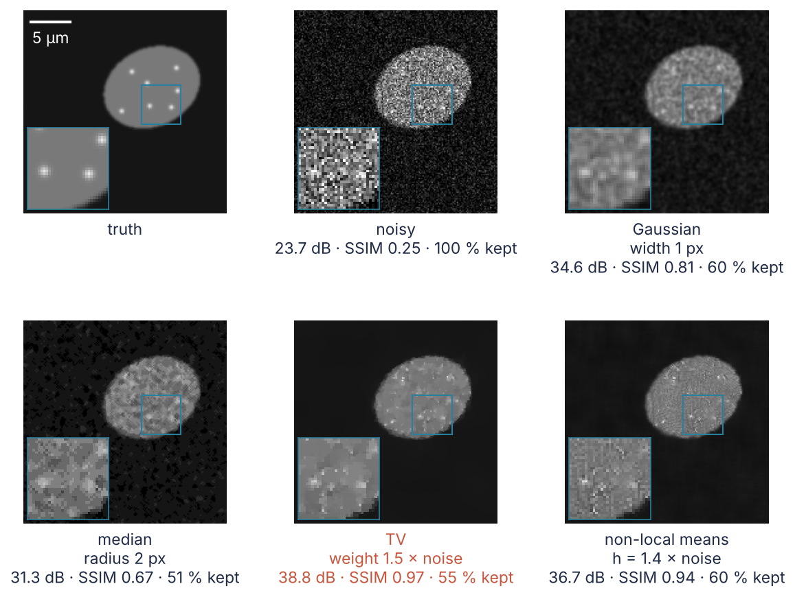
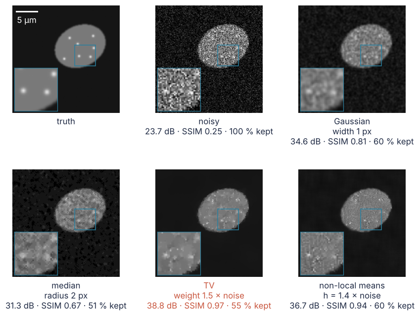
This is where we end up: one cell as it truly is, as the camera recorded it, and after each filter at the setting this tutorial chooses, with a zoom on three spots; Step 6 draws it. Tuned for the best PSNR, the usual global score (Step 2 explains it and SSIM), each filter keeps only 23 to 30 % of the spots' contrast. Tuned to keep at least half of it, TV wins with 38.8 dB against 23.7 dB for the raw image. The settings are chosen without the truth, from marks on the spots, so the same code chooses them on your own image.

Setup

The cell below makes the image: nine elliptical cells blurred by 1 px, forty spots at least 8 px inside a cell, and Poisson counts drawn from the expected photon number lam, stored as uint16 the way a camera file holds them. It keeps lam as the truth, the spot centers sy, sx, and cell_mask. Random numbers with numpy.random explains the seeded generator, so you can run the cell without reading it.

The tools of Counting cells with scipy.ndimage are the base. scikit-image builds on them (filters.gaussian runs scipy.ndimage underneath and gives the same result except at the border) and adds the denoisers, the scores, and one convention for float images that all of them share. estimate_sigma and denoise_wavelet need PyWavelets: pip install scikit-image PyWavelets.

import numpy as np
import matplotlib.pyplot as plt
from scipy import ndimage as ndi
from skimage import filters, metrics, restoration, util
from skimage.morphology import disk

N = 512                          # image size in pixels
px = 0.1625                      # µm per pixel: a 6.5 µm camera pixel behind a 40× objective
background, cell_level, spot_peak = 1, 5, 5      # photons per pixel
rng = np.random.default_rng(7)
rows, cols = np.indices((N, N))

centers, cell_mask, cells = [], np.zeros((N, N), bool), np.zeros((N, N))
while len(centers) < 9:                          # elliptical cells, centers at least 75 px apart
    c = rng.uniform(50, N - 50, 2)
    if any(np.hypot(*(c - c2)) < 75 for c2 in centers):
        continue
    a, b, phi = rng.uniform(34, 44), rng.uniform(24, 32), rng.uniform(0, np.pi)
    u = (rows - c[0]) * np.cos(phi) + (cols - c[1]) * np.sin(phi)
    v = (cols - c[1]) * np.cos(phi) - (rows - c[0]) * np.sin(phi)
    inside = (u / a)**2 + (v / b)**2 <= 1
    if (inside & cell_mask).any():
        continue
    centers.append(c)
    cell_mask |= inside
    cells[inside] = rng.uniform(0.8, 1.0)        # each cell its own brightness
cells = ndi.gaussian_filter(cells, 1.0)          # optical blur

iy, ix = np.nonzero(ndi.distance_transform_edt(cell_mask) >= 8)
sy, sx = [], []
while len(sy) < 40:                              # spots 8 px inside a cell, 12 px apart
    i = rng.integers(len(iy))
    if all(np.hypot(iy[i] - y, ix[i] - x) >= 12 for y, x in zip(sy, sx)):
        sy.append(iy[i])
        sx.append(ix[i])
sy, sx = np.array(sy), np.array(sx)
points = np.zeros((N, N))
points[sy, sx] = 1
spots = ndi.gaussian_filter(points, 1.3)
spots /= spots.max()                             # peak 1, before scaling to photons

lam = background + cell_level * cells + spot_peak * spots    # expected photons: the truth
counts = rng.poisson(lam).astype(np.uint16)                   # what the camera file holds

plt.rcParams.update({
    "figure.figsize": (7, 3.6), "figure.dpi": 110,
    "axes.spines.top": False, "axes.spines.right": False,
    "axes.grid": True, "grid.alpha": 0.25,
    "font.size": 11, "lines.linewidth": 1.8,
})
INK, ACCENT, SECOND, MUTED = "#1f2a44", "#c8553d", "#2a7f9e", "#8a8f98"

print(f"{N} × {N} pixels, {len(centers)} cells covering {100 * cell_mask.mean():.0f} % of the field, "
      f"{len(sy)} spots, mean {lam.mean():.1f} photons per pixel")

512 × 512 pixels, 9 cells covering 12 % of the field, 40 spots, mean 1.5 photons per pixel

Step 1: Convert the counts to floats and measure the noise

Look at the photon counts outside and inside the cells:

print(f"{counts.dtype}, counts from {counts.min()} to {counts.max()}")
for name, where in [("background", ~cell_mask), ("cells", cell_mask)]:
    c = counts[where]
    print(f"{name:10s}  mean {c.mean():.1f}  std {c.std():.1f}  √mean {np.sqrt(c.mean()):.1f}  photons")

uint16, counts from 0 to 19
background  mean 1.0  std 1.0  √mean 1.0  photons
cells       mean 5.5  std 2.4  √mean 2.3  photons

In the background the mean and the standard deviation are both 1.0 photon; inside the cells the counts scatter by 2.4 around 5.5, whose square root is 2.3. A standard deviation equal to the square root of the mean is the mark of Poisson noise. It grows with the brightness.

scikit-image's convention for float images is the range 0 to 1. Its defaults assume it, weight=0.1 and h=0.1 among them, and util.img_as_float maps integer images into it, dividing by the largest value the type can hold:

print(f"img_as_float maximum: {util.img_as_float(counts).max():.5f}")

ceiling = counts.max()           # the largest count in this image
noisy = counts / ceiling
clean = lam / ceiling            # the truth on the same scale

img_as_float maximum: 0.00029

For a uint16 that is 65,535, and the image ends up in the bottom 0.03 % of the range. Divide by the image's largest count instead, 19 here, or for a series by the largest count of the series, so that all images share one scale. The exact ceiling matters little: every knob below is set as a multiple of the noise level, and the noise level scales with the ceiling.

restoration.estimate_sigma measures the noise level from the image's finest wavelet details, the differences between neighboring pixels. Away from edges these are pure noise, and a median over all of them ignores the few edges:

noise = restoration.estimate_sigma(noisy)
err = noisy - clean
print(f"estimate_sigma: {noise:.4f}  ({noise * ceiling:.2f} photons)")
print(f"true noise:     {err[~cell_mask].std():.4f} in the background, {err[cell_mask].std():.4f} in the cells")

estimate_sigma: 0.0559  (1.06 photons)
true noise:     0.0529 in the background, 0.1240 in the cells

The estimate is the background's noise, because the background is 88 % of the field. Inside the cells the noise is 2.3 times larger, which comes back in the first pitfall.

Copy

crop = np.s_[100:260, 312:472]                   # 160 px, 26 µm, around one cell
extent = [0, 160 * px, 160 * px, 0]
fig, axes = plt.subplots(1, 2, figsize=(7, 3.4), sharey=True)
for ax, img, name in zip(axes, [counts, lam], ["noisy", "truth"]):
    im = ax.imshow(img[crop], cmap="gray", vmin=0, vmax=12, extent=extent)
    ax.text(0.04, 0.05, name, color="white", transform=ax.transAxes)
    ax.set(xlabel="x / µm")
    ax.grid(False)
axes[0].set(ylabel="y / µm")
fig.colorbar(im, ax=axes, label="photons per pixel", shrink=0.8, pad=0.03)
plt.show()

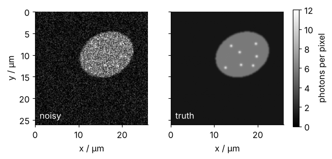
The cell shows through the noise. Its spots do not.

Step 2: Score a filter by the spots it keeps, and by PSNR and SSIM

The number that chooses a setting here is the share of the spots' contrast that a filter keeps. Mark the 40 spot centers in a boolean image at_spot. The distance transform on its inverse gives every pixel its distance to the nearest center, the way the prerequisite's split of touching cells used markers == 0, and the pixels 4 to 6 px away form a ring that measures the local level around each spot.

The contrast of an image is its mean at the centers minus its mean on the rings, and "kept" divides a filter's contrast by the raw image's. The rule, coded as pick, takes the strongest setting that keeps at least half the spot contrast. Half is my choice; raise it when the spots matter more.

at_spot = np.zeros((N, N), bool)
at_spot[sy, sx] = True
dist = ndi.distance_transform_edt(~at_spot)      # px to the nearest spot center
ring = (dist >= 4) & (dist <= 6)

def contrast(x, at_spot, ring):
    return x[at_spot].mean() - x[ring].mean()

def score(x, at_spot, ring):
    """PSNR and SSIM against the truth, and the share of the raw spot contrast that x keeps."""
    psnr = metrics.peak_signal_noise_ratio(clean, x, data_range=1)
    ssim = metrics.structural_similarity(clean, x, data_range=1)
    return psnr, ssim, contrast(x, at_spot, ring) / contrast(noisy, at_spot, ring)

def show(setting, x):
    psnr, ssim, kept = score(x, at_spot, ring)
    print(f"{setting:>14s}   PSNR {psnr:4.1f} dB   SSIM {ssim:.2f}   spots kept {100 * kept:3.0f} %")

def pick(runs, at_spot, ring):
    """The strongest setting that keeps at least half the spot contrast."""
    return max(k for k, x in runs.items() if score(x, at_spot, ring)[2] >= 0.5)

print(f"ring: {ring.sum() / at_spot.sum():.0f} px per spot")
print(f"spot contrast: raw {contrast(counts, at_spot, ring):.2f} photons, truth {contrast(lam, at_spot, ring):.2f} photons")
show("noisy image", noisy)

ring: 68 px per spot
spot contrast: raw 5.29 photons, truth 4.99 photons
   noisy image   PSNR 23.7 dB   SSIM 0.25   spots kept 100 %

Over 40 spots the noise averages out: the raw contrast, 5.29 photons, stands in for the truth's 4.99, and the 6 % gap is the uncertainty of the 50 % line.

PSNR compares the mean squared error with the square of the data range \(R\), \(\mathrm{PSNR} = 10\log_{10}(R^2/\mathrm{MSE})\) in dB, so 3 dB more means half the squared error. It ranks filters on one image, not images against each other. SSIM compares local means, variances, and the covariance of the two images in a 7 × 7 window and averages over the image; 1 means identical. Pass data_range to both every time: SSIM refuses floats without it, and peak_signal_noise_ratio silently assumes 1.

PSNR and SSIM need the truth, and the rule needs only the spot centers: here the simulation's, and on your own image marks you set by hand (end of Step 6). There the rule alone chooses; here the truth grades it.

Step 3: Smooth with the Gaussian and the median filter

filters.gaussian is the Gaussian smoothing of the prerequisite. Its width in pixels goes in as sigma, the API's name for it:

gauss = {w: filters.gaussian(noisy, sigma=w) for w in [0.5, 1, 1.5, 2, 3]}
for w, x in gauss.items():
    show(f"width {w} px", x)

  width 0.5 px   PSNR 27.5 dB   SSIM 0.45   spots kept  89 %
    width 1 px   PSNR 34.6 dB   SSIM 0.81   spots kept  60 %
  width 1.5 px   PSNR 37.2 dB   SSIM 0.91   spots kept  39 %
    width 2 px   PSNR 37.9 dB   SSIM 0.94   spots kept  25 %
    width 3 px   PSNR 37.0 dB   SSIM 0.96   spots kept  11 %

PSNR peaks at 2 px with 37.9 dB, where a quarter of the spot contrast is left. The rule picks 1 px: 34.6 dB, with 60 % kept. A line from the background across the cell edge and through a spot shows where the rest went:

Copy

line = np.s_[179, 366:417]                       # through the cell edge and a spot at x = 3.7 µm
x_um = np.arange(51) * px
fig, ax = plt.subplots(figsize=(7, 3.4))
ax.plot(x_um, noisy[line] * ceiling, "o", color=MUTED, ms=4, clip_on=False, label="noisy")
ax.plot(x_um, lam[line], color=INK, label="truth")
for w, alpha in [(1, 0.5), (2, 1.0)]:
    ax.plot(x_um, gauss[w][line] * ceiling, color=ACCENT, alpha=alpha, label=f"width {w} px")
ax.legend(frameon=False, loc="upper left")
ax.set(xlabel="position / µm", ylabel="photons per pixel", xlim=(0, x_um[-1]), ylim=(0, None))
plt.show()

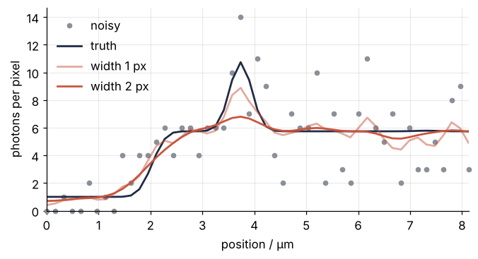
Smoothing turns the edge into a ramp and spreads the spot's peak into its surroundings. The two widths are one color, light for 1 px and dark for 2 px, and in the table 2 px keeps less than half of what 1 px kept.

The median filter replaces each pixel by the middle value of a disk around it, which removes an outlier instead of averaging it in:

median = {r: filters.median(noisy, disk(r)) for r in [1, 2, 3]}
for r, x in median.items():
    show(f"radius {r} px", x)

   radius 1 px   PSNR 28.2 dB   SSIM 0.47   spots kept  76 %
   radius 2 px   PSNR 31.3 dB   SSIM 0.67   spots kept  51 %
   radius 3 px   PSNR 34.3 dB   SSIM 0.84   spots kept  30 %

At every radius its PSNR is lower than that of a Gaussian keeping the same share of the spot contrast. The rule picks radius 2, 31.3 dB with 51 % kept, and radius 3 already falls to 30 %. At 1 to 6 photons the middle of a set of whole counts can only land on a few values, so flat regions break into patches of one level.

Step 4: Average alike patches with non-local means

Non-local means compares the 5 × 5 patch around each pixel with every patch centered up to 6 px away (patch_distance=6, a 13 × 13 window) and averages their centers, with weights that fall as the patches differ. h sets how different still counts as alike. Two noisy copies of the same patch differ by the noise alone; passing the noise level as sigma subtracts that expected difference, so that only a real difference lowers a weight. Here sigma is the noise level, under the keyword that filters.gaussian uses for a width.

nlm = {k: restoration.denoise_nl_means(noisy, h=k * noise, sigma=noise, patch_size=5, patch_distance=6)
       for k in [1.0, 1.2, 1.4, 1.6, 1.8, 2.0]}
for k, x in nlm.items():
    show(f"h = {k} × noise", x)

h = 1.0 × noise   PSNR 31.8 dB   SSIM 0.91   spots kept  96 %
h = 1.2 × noise   PSNR 34.6 dB   SSIM 0.93   spots kept  81 %
h = 1.4 × noise   PSNR 36.7 dB   SSIM 0.94   spots kept  60 %
h = 1.6 × noise   PSNR 37.9 dB   SSIM 0.95   spots kept  41 %
h = 1.8 × noise   PSNR 38.4 dB   SSIM 0.96   spots kept  29 %
h = 2.0 × noise   PSNR 38.5 dB   SSIM 0.96   spots kept  23 %

The rule picks h = 1.4 × noise level: 36.7 dB, 60 % kept. PSNR is still rising at 2.0 ×, 38.5 dB with 23 % left. The best multiple lies above 1 because the noise level is the background's, and the cells are noisier.

Step 5: Sweep the total variation weight

TV denoising looks for the image closest to the noisy one whose total variation, the summed size of all its jumps, is small, and weight sets the trade between the two. A flat region costs nothing. An edge costs its height times its length, so a few long edges survive and the noise does not. A small spot has a long rim for its area, so it fades first.

The function improves its answer in rounds and by default stops when a round changes little, at a different stage for each weight. eps=1e-12 switches that stop off and max_num_iter=300 gives every weight the same 300 rounds:

tv_runs = {k: restoration.denoise_tv_chambolle(noisy, weight=k * noise, eps=1e-12, max_num_iter=300)
           for k in [0.75, 1, 1.25, 1.5, 1.75, 2, 2.5, 3, 3.5, 4]}
for k, x in tv_runs.items():
    show(f"{k} × noise", x)
print(f"weight 1.5 × noise level = {1.5 * noise:.3f} in image units")

  0.75 × noise   PSNR 32.5 dB   SSIM 0.88   spots kept  80 %
     1 × noise   PSNR 35.0 dB   SSIM 0.93   spots kept  72 %
  1.25 × noise   PSNR 37.1 dB   SSIM 0.95   spots kept  64 %
   1.5 × noise   PSNR 38.8 dB   SSIM 0.97   spots kept  55 %
  1.75 × noise   PSNR 40.0 dB   SSIM 0.98   spots kept  47 %
     2 × noise   PSNR 40.6 dB   SSIM 0.98   spots kept  39 %
   2.5 × noise   PSNR 40.7 dB   SSIM 0.99   spots kept  25 %
     3 × noise   PSNR 40.2 dB   SSIM 0.99   spots kept  14 %
   3.5 × noise   PSNR 39.7 dB   SSIM 0.98   spots kept   7 %
     4 × noise   PSNR 39.3 dB   SSIM 0.98   spots kept   4 %
weight 1.5 × noise level = 0.084 in image units

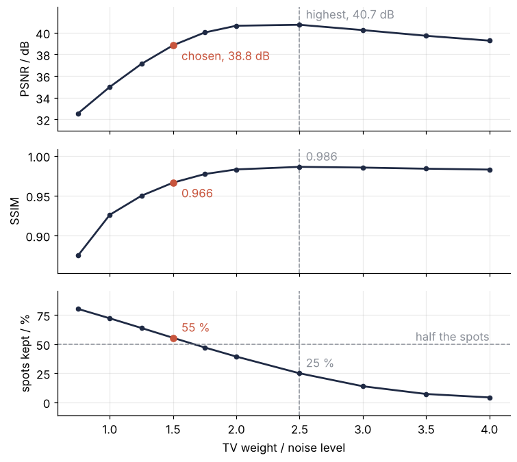
The rule picks 1.5 ×: 38.8 dB, with 55 % kept. In image units that weight is 0.084, the number a methods section would print and the second pitfall copies to another image.

Copy

ks = np.array(list(tv_runs))
tv_scores = np.array([score(x, at_spot, ring) for x in tv_runs.values()])
i_pick = list(tv_runs).index(pick(tv_runs, at_spot, ring))
i_best = tv_scores[:, 0].argmax()                # the highest PSNR
panels = [("PSNR / dB", tv_scores[:, 0], "chosen, {:.1f} dB", "highest, {:.1f} dB", -14),
          ("SSIM", tv_scores[:, 1], "{:.3f}", "{:.3f}", -14),
          ("spots kept / %", 100 * tv_scores[:, 2], "{:.0f} %", "{:.0f} %", 6)]
fig, axes = plt.subplots(3, 1, figsize=(7, 6.3), sharex=True)
for ax, (label, values, at_pick, at_best, dy) in zip(axes, panels):
    ax.axvline(ks[i_best], color=MUTED, ls="--", lw=1)
    ax.plot(ks, values, "o-", color=INK, ms=4)
    ax.plot(ks[i_pick], values[i_pick], "o", color=ACCENT, ms=6)
    ax.annotate(at_pick.format(values[i_pick]), (ks[i_pick], values[i_pick]), xytext=(8, dy),
                textcoords="offset points", color=ACCENT)
    ax.annotate(at_best.format(values[i_best]), (ks[i_best], values[i_best]), xytext=(6, 6),
                textcoords="offset points", color=MUTED)
    ax.set(ylabel=label)
    ax.margins(y=0.2)
axes[0].set(yticks=range(32, 42, 2))
axes[2].axhline(50, color=MUTED, ls="--", lw=1)
axes[2].text(4.0, 53, "half the spots", color=MUTED, ha="right")
axes[2].set(xlabel="TV weight / noise level")
fig.tight_layout()
plt.show()
print(f"pixels within 3 px of a spot center: {100 * (dist <= 3).mean():.2f} % of the image")

pixels within 3 px of a spot center: 0.44 % of the image

PSNR and SSIM both peak at 2.5 × (40.7 dB and 0.986), where a quarter of the spot contrast is left. A global score misses this because the spots are a small part of the image: the pixels within 3 px of a center are 0.44 % of the field, so erasing them barely moves an average over all of it. SSIM, often recommended over PSNR, is no cure. Over the Gaussian widths of Step 3 it is still rising at 3 px, where 11 % of the spot contrast is left.

Step 6: Compare the four filters at their best

The rule's picks from the four sweeps, and a fifth contender: restoration.denoise_wavelet splits the image into details at several scales, sets the small ones, mostly noise, to zero, shrinks the rest, and rebuilds the image. Here it estimates its noise level sigma itself, the way most people call it.

w, r, k, h = (pick(runs, at_spot, ring) for runs in [gauss, median, tv_runs, nlm])
results = {
    "Gaussian": (f"width {w} px", gauss[w]),
    "median": (f"radius {r} px", median[r]),
    "TV": (f"weight {k} × noise", tv_runs[k]),
    "non-local means": (f"h = {h} × noise", nlm[h]),
    "wavelet": ("automatic", restoration.denoise_wavelet(noisy)),
}
print(f"{'filter':15s}  {'setting':18s}  PSNR      SSIM  spots kept")
for name, (setting, x) in results.items():
    psnr, ssim, kept = score(x, at_spot, ring)
    print(f"{name:15s}  {setting:18s}  {psnr:4.1f} dB   {ssim:.2f}  {100 * kept:3.0f} %")

filter           setting             PSNR      SSIM  spots kept
Gaussian         width 1 px          34.6 dB   0.81   60 %
median           radius 2 px         31.3 dB   0.67   51 %
TV               weight 1.5 × noise  38.8 dB   0.97   55 %
non-local means  h = 1.4 × noise     36.7 dB   0.94   60 %
wavelet          automatic           36.1 dB   0.94   19 %

TV wins under the rule and non-local means comes second. The Gaussian keeps as much of the spot contrast as non-local means, 60 %, and pays for it in a background that stays grainy. The wavelet denoiser picks its own cutoffs and gives the spots away: 36.1 dB, but 19 % kept. Sweep its sigma under the rule before you trust it. In every sweep the rule's pick is also the setting with the highest PSNR among those that keep half, so the truth agrees with a choice made without it.

Copy

zy, zx, zw = 159, 405, 31                        # the zoom square, 5 µm on a side
panels = [("truth", "", clean), ("noisy", "", noisy)] + [
    (name, setting, x) for name, (setting, x) in results.items() if name != "wavelet"]
y0, x0 = crop[0].start, crop[1].start           # the crop's corner in the full image
fig, axes = plt.subplots(2, 3, figsize=(8, 6.4))
for ax, (name, setting, x) in zip(axes.flat, panels):
    ax.imshow(x[crop] * ceiling, cmap="gray", vmin=0, vmax=12, extent=extent)
    ax.add_patch(plt.Rectangle(((zx - x0) * px, (zy - y0) * px), zw * px, zw * px,
                               fill=False, ec=SECOND, lw=1))
    inset = ax.inset_axes([0.02, 0.02, 0.4, 0.4])
    inset.imshow(x[zy:zy + zw, zx:zx + zw] * ceiling, cmap="gray", vmin=0, vmax=12)
    inset.set(xticks=[], yticks=[])
    for side in inset.spines.values():
        side.set(visible=True, color=SECOND)
    ax.set_axis_off()
    label = f"{name}\n{setting}" if setting else name
    if name != "truth":                          # nothing to score against itself
        psnr, ssim, kept = score(x, at_spot, ring)
        label += f"\n{psnr:.1f} dB · SSIM {ssim:.2f} · {100 * kept:.0f} % kept"
    ax.text(0.5, -0.03, label, transform=ax.transAxes, ha="center", va="top",
            color=ACCENT if name == "TV" else INK)
axes[0, 0].plot([1, 6], [1.5, 1.5], color="white", lw=2)    # a 5 µm scale bar
axes[0, 0].text(3.5, 2.3, "5 µm", color="white", ha="center", va="top")
fig.tight_layout()
plt.show()

On your own image, take a second exposure of the same field right after the first, smooth it with a Gaussian of width 1 px, and mark 30 or more spots on it by hand in Fiji or napari, not on the image you denoise (the third pitfall shows why). The marks hold only where the spots sit in the same place in both exposures, as they do in a fixed sample. at_spot[ys, xs] = True turns them into the mask, with rows first and in pixels; Fiji lists x first, and in µm when the image is calibrated. Fewer spots than 40 widen the uncertainty around the 50 % line. This still-field route is the only one tested here: for spots that move between exposures, or a single image you cannot repeat, the tutorial has no measure. For edges or texture, start from the residual in Variations.

Pitfalls

Poisson noise treated as Gaussian. After the chosen non-local means the background is smooth and the cells are still grainy. The residual says by how much:

err = (nlm[h] - clean) * ceiling                 # in photons
print(f"residual: {err[~cell_mask].std():.2f} photons in the background, {err[cell_mask].std():.2f} in the cells")

residual: 0.10 photons in the background, 0.74 in the cells

Seven times more inside the cells, and you see it without any truth in the final figure. The cause is one noise level, the background's, for noise that grows as the square root of the signal (Step 1). Stabilize the variance first with the Anscombe transform (Variations), or estimate the noise level in a region inside a cell.

A weight copied from another image. A TV weight from a paper, or from your last image, is a number in someone else's brightness units:

noisy30 = counts / 30                            # the same counts, another ceiling
tv30 = restoration.denoise_tv_chambolle(noisy30, weight=1.5 * noise, eps=1e-12, max_num_iter=300)
kept30 = contrast(tv30, at_spot, ring) / contrast(noisy30, at_spot, ring)
print(f"weight {1.5 * noise:.3f} on counts / 30: spots kept {100 * kept30:.0f} %")

f = util.img_as_float(counts)
tv_default = restoration.denoise_tv_chambolle(f)
kept_default = contrast(tv_default, at_spot, ring) / contrast(f, at_spot, ring)
print(f"default weight 0.1 on img_as_float: {0.1 / restoration.estimate_sigma(f):,.0f} × its noise level, "
      f"spots kept {100 * kept_default:.0f} %")

weight 0.084 on counts / 30: spots kept 28 %
default weight 0.1 on img_as_float: 6,169 × its noise level, spots kept 2 %

The weight that kept 55 % here keeps 28 % on the same counts divided by 30 instead of 19. The default on img_as_float is 6,169 times that image's noise level and leaves 2 % of the spots. weight and h are in the image's brightness units, which depend on how the counts were scaled. Set them as multiples of estimate_sigma of the image at hand, as Steps 4 and 5 do.

Marking the spots on the noisy image. Here marking by eye is simulated by the 40 brightest tops inside the cells, found with the prerequisite's maximum_filter test: once on the noisy image, once on a second exposure of the same field smoothed by 1 px. Each set of marks gets its own mask and ring:

second = rng.poisson(lam) / ceiling              # a second exposure of the same field

def mark(img, n=40):
    """The n brightest tops inside the cells."""
    ty, tx = np.nonzero((img == ndi.maximum_filter(img, size=13)) & cell_mask)
    order = np.argsort(-img[ty, tx], kind="stable")[:n]
    return ty[order], tx[order]

for name, img in [("noisy image", noisy), ("second exposure", filters.gaussian(second, sigma=1))]:
    ty, tx = mark(img)
    marks = np.zeros((N, N), bool)
    marks[ty, tx] = True
    d = ndi.distance_transform_edt(~marks)
    ring_m = (d >= 4) & (d <= 6)
    print(f"{name:15s}  {(dist[ty, tx] <= 2).sum()} of 40 on a spot   contrast raw {contrast(counts, marks, ring_m):4.1f}, "
          f"truth {contrast(lam, marks, ring_m):.1f} photons   picks: TV {pick(tv_runs, marks, ring_m)} × noise, "
          f"Gaussian {pick(gauss, marks, ring_m)} px")

noisy image      17 of 40 on a spot   contrast raw 10.1, truth 1.7 photons   picks: TV 1.25 × noise, Gaussian 0.5 px
second exposure  32 of 40 on a spot   contrast raw  4.0, truth 3.3 photons   picks: TV 1.5 × noise, Gaussian 1 px

On the noisy image 17 of 40 marks lie on a spot. At the marks the raw image stands 10.1 photons above its rings and the truth 1.7, and the rule stops at TV 1.25 × and the Gaussian at 0.5 px. The brightest-looking pixels of a noisy image are mostly noise peaks, so the marks select noise and inflate the reference; every filter removes noise, so every filter seems to lose spots. The marks on the second exposure find 32 spots and give the picks of the true centers, 1.5 × and 1 px. Mark on a second exposure, as Step 6 describes.

Variations

• Anscombe before a denoiser built for Gaussian noise. A = 2 * np.sqrt(counts + 3/8) brings the noise level close to 1 everywhere, a little lower in the dark background. Denoise A with h and sigma set from estimate_sigma(A) as in Step 4, then invert with \((y/2)^2 - 1/8\), or at counts this low with the exact unbiased inverse of Mäkitalo and Foi, which their paper gives and scikit-image does not. The transform wants photoelectrons, and a camera file holds analog-to-digital units (ADU): subtract the offset and divide by the gain in ADU per electron, both from the data sheet.
• A 3D stack. All four filters take 3D arrays. With voxels taller than they are wide, give filters.gaussian one width per axis, sigma=(0.5, 2, 2). Non-local means gets slow in 3D, so crop first.
• Look at what was removed. The residual noisy - denoised, the method noise, should look like noise, with no cell outlines and no spots in it. It is the picture to check next to the spot measure.
• Deconvolution. When the optical blur hides the spots more than the noise does, restoration.richardson_lucy is the tool (planned tutorial).

Cheat sheet

noisy = counts / counts.max()                         # floats from 0 to 1
noise = restoration.estimate_sigma(noisy)             # noise level, a standard deviation
g = filters.gaussian(noisy, sigma=1)                  # sigma here is a width in px
m = filters.median(noisy, disk(2))                    # disk radius in px
nl = restoration.denoise_nl_means(noisy, h=1.4 * noise, sigma=noise, patch_size=5, patch_distance=6)
tv = restoration.denoise_tv_chambolle(noisy, weight=1.5 * noise, eps=1e-12, max_num_iter=300)
dist = ndi.distance_transform_edt(~at_spot)           # at_spot[ys, xs] = True at marked spots
ring = (dist >= 4) & (dist <= 6)                      # the local level around each spot
kept = (tv[at_spot].mean() - tv[ring].mean()) / (noisy[at_spot].mean() - noisy[ring].mean())
psnr = metrics.peak_signal_noise_ratio(clean, tv, data_range=1)   # only with a truth

Further reading

• The scikit-image user guide and the API pages of skimage.restoration and skimage.metrics.
• Rudin, Osher, and Fatemi, Physica D 60, 259 (1992), for total variation; Chambolle, J. Math. Imaging Vis. 20, 89 (2004), for the algorithm behind denoise_tv_chambolle; Buades, Coll, and Morel, CVPR (2005), for non-local means; Wang et al., IEEE Trans. Image Process. 13, 600 (2004), for SSIM; Mäkitalo and Foi, IEEE Trans. Image Process. 20, 99 (2011), for the Anscombe inverse.
• Bankhead, Introduction to Bioimage Analysis, for noise in microscope images, and Gonzalez and Woods, Digital Image Processing, for the filters.
• Related tutorials on this site: Counting cells with scipy.ndimage: how many are there, and how large?, the step after denoising; Counting cells with JuliaImages, the same in Julia; Random numbers with numpy.random; Filtering with scipy.signal: mains hum and noise out of an ECG, the same trade of noise against detail in one dimension; MRI k-space reconstruction with numpy.fft, images whose artifacts come from sampling, not shot noise; Zoom into a detail of a Matplotlib plot with an inset, for the zooms of the final figure; Colormaps: why a rainbow scale draws features that are not in the data, for why the images are gray. Planned: deconvolution and background removal of microscope images.
• Download the notebook. It was executed with the library versions in the header.