MRI k-space reconstruction with numpy.fft: shifts, fold-over, ringing

The problem: what an MRI scanner actually measures

An MRI scanner does not take a picture. For each slice it measures k-space, the two-dimensional Fourier transform of the slice, and it measures it one row at a time: 256 rows of 256 complex samples is a common size. In a conventional spin-echo or gradient-echo sequence each row costs one repetition of the pulse sequence, a few milliseconds to a few seconds depending on the contrast. Faster sequences take several rows per repetition, and in all of them the scan time is proportional to the number of rows. Measure 128 rows and the scan takes half as long. The question is what the image looks like then, and why.

The field has its own words for the two directions. A gradient field makes the spins precess faster with growing \(x\), so while it is on, their phase winds up like a Fourier probe of growing \(k_x\), and the scanner samples one row along it in a few milliseconds; that row is called a line, its sampling the readout, and it runs horizontally, one sample per column of the array. Between lines the scanner steps \(k_y\) with a short gradient pulse, the phase encode, and waits for the next repetition; that is the vertical direction, from row to row. Samples along a line are nearly free.

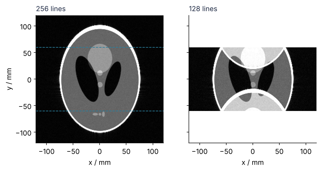
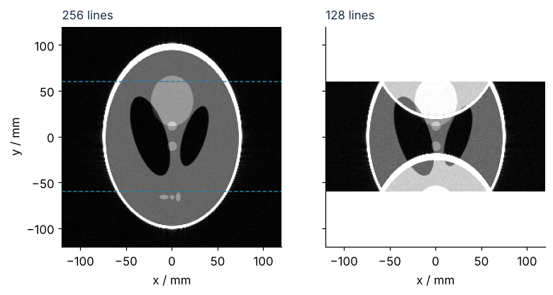
On the left is the head reconstructed from all 256 lines, on the right the same head from every second line: the image is half as tall, and the top and bottom of the skull have folded into the brain. The last step draws this figure. The data are simulated, a standard head phantom of ten ellipses whose Fourier transform is known exactly, sampled the way a scanner samples it and with noise added.

Setup

Everything below the data generation comment builds the phantom's k-space and is not part of the method; your own scan replaces kspace. A raw file, in a vendor format or ISMRMRD, holds complex samples for each receive coil and is read with that format's own tools. What the steps need is one coil and one 2D Cartesian slice as a complex array, lines on axis 0 and readout samples on axis 1 (transpose if not). If the protocol oversampled the readout by two, the image comes out twice as wide as the field of view: keep its middle half of columns.

import numpy as np
import matplotlib.pyplot as plt
from scipy.special import j1

N = 256            # samples per line and number of lines
FOV = 240.0        # field of view / mm
dx = FOV / N       # pixel size / mm

plt.rcParams.update({
    "figure.figsize": (7, 3.6), "figure.dpi": 110,
    "axes.spines.top": False, "axes.spines.right": False,
    "axes.grid": True, "grid.alpha": 0.25,
    "font.size": 11, "lines.linewidth": 1.8,
})
INK, ACCENT, SECOND, MUTED = "#1f2a44", "#c8553d", "#2a7f9e", "#8a8f98"

# ---- data generation: replace kspace with your own centered array
# Modified Shepp-Logan phantom (Toft 1996): intensity, semi-axes a and b, center x0 and y0, angle in degrees
ELLIPSES = np.array([
    [ 1.0, 0.6900, 0.9200,  0.00,  0.0000,   0],
    [-0.8, 0.6624, 0.8740,  0.00, -0.0184,   0],
    [-0.2, 0.1100, 0.3100,  0.22,  0.0000, -18],
    [-0.2, 0.1600, 0.4100, -0.22,  0.0000,  18],
    [ 0.1, 0.2100, 0.2500,  0.00,  0.3500,   0],
    [ 0.1, 0.0460, 0.0460,  0.00,  0.1000,   0],
    [ 0.1, 0.0460, 0.0460,  0.00, -0.1000,   0],
    [ 0.1, 0.0460, 0.0230, -0.08, -0.6050,   0],
    [ 0.1, 0.0230, 0.0230,  0.00, -0.6060,   0],
    [ 0.1, 0.0230, 0.0460,  0.06, -0.6050,   0],
])
ELLIPSES[:, 1:5] *= 110.0                                 # to mm: a head about 200 mm tall

def phantom_kspace(kx, ky):
    """Exact Fourier transform of the ellipses at kx, ky in 1/mm. Data generation only."""
    F = np.zeros(kx.shape, dtype=complex)
    for rho, a, b, x0, y0, phi in ELLIPSES:
        c, s = np.cos(np.radians(phi)), np.sin(np.radians(phi))
        K = np.hypot(a * (kx * c + ky * s), b * (-kx * s + ky * c))
        K_safe = np.where(K == 0, 1.0, K)
        # ellipse transform a b J1(2 pi K) / K, with its limit pi a b at K = 0; not needed for your data
        shape = np.where(K == 0, np.pi * a * b, a * b * j1(2 * np.pi * K_safe) / K_safe)
        F += rho * shape * np.exp(-2j * np.pi * (kx * x0 + ky * y0))
    return F

k = (np.arange(N) - N // 2) / FOV                          # sorted, zero at index N/2, as a scanner stores it
KX, KY = np.meshgrid(k, k)
# echo 2 samples late along kx; dividing by dx**2 puts the image in phantom units (data generation only)
kspace_clean = phantom_kspace(KX - 2 / FOV, KY) / dx**2
rng = np.random.default_rng(1)
# noise of 0.0075 in the real and in the imaginary part of the image needs 0.0075 * N in k-space (data generation only)
kspace = kspace_clean + 0.0075 * N * (rng.standard_normal((N, N)) + 1j * rng.standard_normal((N, N)))

print(kspace.shape, kspace.dtype)

(256, 256) complex128

Step 1: Look at k-space and find its center

Rows are lines, columns are readout samples. The values span many orders of magnitude, so plot the logarithm of the magnitude, the whole array and a zoom on its middle:

Copy

center = np.unravel_index(np.abs(kspace).argmax(), kspace.shape)
fig, axes = plt.subplots(1, 2, figsize=(8, 3.8), layout="constrained")
for ax, half_width, ticks in zip(axes, [N // 2, 8], [[0, 64, 128, 192, 256], [120, 124, 128, 132]]):
    im = ax.imshow(np.log10(np.abs(kspace)), cmap="gray", origin="lower")
    ax.axhline(N // 2, color=MUTED, lw=1)
    ax.axvline(N // 2, color=MUTED, lw=1)
    ax.plot(center[1], center[0], "o", color=ACCENT, ms=6 if half_width == 8 else 4)
    ax.set(xlim=(N // 2 - half_width - 0.5, N // 2 + half_width - 0.5),
           ylim=(N // 2 - half_width - 0.5, N // 2 + half_width - 0.5),
           xticks=ticks, yticks=ticks, xlabel="readout sample ($k_x$)")
    ax.grid(False)
axes[0].set(ylabel="line ($k_y$)")
fig.colorbar(im, ax=axes, label="log₁₀ |k-space|", shrink=0.85)
plt.show()

print("brightest sample at (line, column) =", tuple(int(i) for i in center))

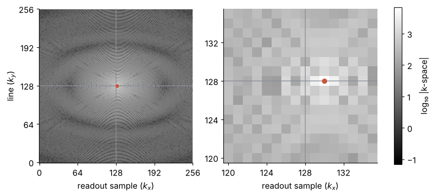
brightest sample at (line, column) = (128, 130)

The center of k-space is zero frequency, where the Fourier probe is a constant and the sample is the sum over the whole slice. For an object that is not mostly negative, that is by far the largest sample, so argmax finds it. Row 128 is \(N/2\): the lines are centered, which is how scanners store them and what this tutorial assumes. Column 130 is two samples off, an echo that arrives slightly late, as it often does on a real scanner; Step 3 shows what that does to the image. Run the same test on your own data. If the brightest sample sits at a corner, near (0, 0), the data are already in NumPy's order, and the end of Step 2 gives the call for that case.

Step 2: Reconstruct with ifftshift, ifft2, fftshift

The prerequisite used rfft, which keeps zero and the positive frequencies only. The full FFT keeps the negative ones too and stores them in an order of its own. fftfreq shows it, here for eight samples:

print("NumPy order:", np.fft.fftfreq(8))
print("sorted:     ", np.fft.fftshift(np.fft.fftfreq(8)))

NumPy order: [ 0.     0.125  0.25   0.375 -0.5   -0.375 -0.25  -0.125]
sorted:      [-0.5   -0.375 -0.25  -0.125  0.     0.125  0.25   0.375]

Zero comes first, then the positive frequencies, then the negative ones from the most negative upward. fftshift sorts them, with zero at index \(N/2 = 4\). A scanner delivers k-space sorted, and ifft2 expects NumPy's order, so the reconstruction is three calls. ifftshift takes the data from sorted to NumPy's order. ifft2 transforms back along both axes, which is nothing more than a 1D inverse transform of every row, then of every column. ifft2 returns the image positions in the same circular order as fftfreq, \(x = 0\) first, and fftshift sorts them:

Copy

def recon(k):
    return np.fft.fftshift(np.fft.ifft2(np.fft.ifftshift(k)))

image = recon(kspace)
print(image.shape, image.dtype, f"max |image| = {np.abs(image).max():.2f}")

extent = [-FOV / 2, FOV / 2, -FOV / 2, FOV / 2]
fig, ax = plt.subplots(figsize=(4.4, 4))
ax.imshow(np.abs(image), cmap="gray", vmin=0, vmax=0.5, origin="lower", extent=extent)
ax.set(xlabel="x / mm", ylabel="y / mm")
ax.grid(False)
plt.show()

(256, 256) complex128 max |image| = 1.13

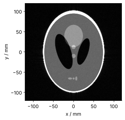
The image is complex, and its magnitude is the head. The gray scale stops at 0.5 so that the brain, at 0.2, shows its structure; the skull saturates. Its true intensity is 1.00, and the maximum of 1.13 is above it: the noiseless data already reach 1.115, for a reason Step 4 gives, and noise adds the rest.

For even \(N\) the two shifts are the same permutation. For odd \(N\) they are not:

print("fftshift: ", np.fft.fftshift(np.arange(5)), "  ifftshift:", np.fft.ifftshift(np.arange(5)))

fftshift:  [3 4 0 1 2]   ifftshift: [2 3 4 0 1]

They differ by one place, and the order in recon is right for both. The two shifts also do separate jobs: ifftshift is about the order of the data, fftshift about where the image's center is shown. For data whose brightest sample sits at a corner, drop the first and keep the second, np.fft.fftshift(np.fft.ifft2(k)).

Step 3: Read the phase, and why plotting the real part fails

The head is real, and still the image is complex. The cause is the late echo. Shifting k-space by \(\mathbf k_0\) multiplies the image by a phase that turns linearly with position: if \(F(\mathbf k)\) is the Fourier transform of \(m(\mathbf x)\), then

This is the shift theorem, and the prerequisite's lost phase is the same phase in one dimension. The data are shifted by \(k_0 = 2/\text{FOV}\) along \(k_x\), so the phase makes two full turns across the 240 mm:

Copy

head = np.abs(image) > 0.05                       # phase of the empty background is noise
fig, axes = plt.subplots(1, 3, figsize=(8, 3.1), sharey=True, layout="constrained")
axes[0].imshow(np.abs(image), cmap="gray", vmin=0, vmax=0.5, origin="lower", extent=extent)
axes[1].imshow(image.real, cmap="RdBu_r", vmin=-0.5, vmax=0.5, origin="lower", extent=extent)
axes[2].imshow(np.where(head, np.angle(image), np.nan), cmap="twilight", vmin=-np.pi, vmax=np.pi,
               origin="lower", extent=extent)
for ax, label in zip(axes, ["magnitude", "real part", "phase"]):
    ax.text(0, 1.02, label, transform=ax.transAxes, va="bottom", color=INK)
    ax.set(xlabel="x / mm", xticks=[-100, 0, 100], yticks=[-100, 0, 100])
    ax.grid(False)
axes[0].set(ylabel="y / mm")
plt.show()

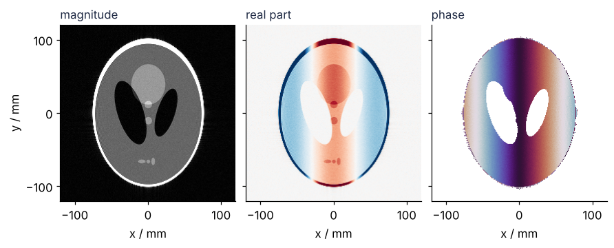
The real part is the magnitude times the cosine of the ramp: vertical bands, half of them negative. That is neither a feature of the head nor a bug. To measure the ramp, multiply each pixel by the conjugate of its left neighbor and sum over the bright pixels of the head. The angle of \(z_{j+1}\bar z_j\) is the phase step itself, while differences of np.angle jump by \(2\pi\) at each of the two wraps:

x = (np.arange(N) - N // 2) * dx                  # pixel positions / mm, same for y
bright = (np.abs(image) > 0.15)[:, 1:] & (np.abs(image) > 0.15)[:, :-1]
step = np.angle(np.sum((image[:, 1:] * np.conj(image[:, :-1]))[bright]))
print(f"phase ramp: {step * N / (2 * np.pi):.2f} cycles across the field of view")

corrected = image * np.exp(-2j * np.pi * (2 / FOV) * x)   # undo the 2-sample offset from Step 1
corrected_clean = recon(kspace_clean) * np.exp(-2j * np.pi * (2 / FOV) * x)
print(f"after correction: max |imaginary part| = {np.abs(corrected.imag).max():.3f}, "
      f"without noise {np.abs(corrected_clean.imag).max():.3f}")

phase ramp: 1.99 cycles across the field of view
after correction: max |imaginary part| = 0.039, without noise 0.012

1.99 cycles, the two samples of Step 1. After the correction the imaginary part is at most 0.039. Without noise it is at most 0.012, left by the sharp edge of the measured k-space that Step 4 takes up. The rest is noise, 0.0075 in each of the two channels, the real and the imaginary part (a receive coil is also called a channel in MRI, but not here). The largest excursion among 65,536 pixels is about four times that. Look at np.abs for the picture, and keep the complex image for the day you need the phase.

Step 4: Cut k-space short, and the ringing at the edges

A scanner measures \(k\) only up to \(\pm N/(2\,\text{FOV})\), here 0.53 per mm, and beyond that the record stops. In the prerequisite, a record of finite length \(T\) smeared every peak of the spectrum into a skirt about \(1/T\) wide. A finite range of \(k\) does the same to the image: every sharp edge is smeared over about a pixel and overshoots, with ripples running away from it. This is Gibbs ringing. Measure it on the noiseless data, at the skull, whose true intensity is 1.00:

hann = np.outer(np.hanning(N), np.hanning(N))
plain = np.abs(recon(kspace_clean))
windowed = np.abs(recon(kspace_clean * hann))
padded = np.abs(recon(np.pad(kspace_clean, N // 2))) * 4   # 512 x 512; ifft2 now divides by 4 times more samples

print(f"maximum, plain:       {plain.max():.3f}")
print(f"maximum, Hann window: {windowed.max():.3f}")
print(f"maximum, zero-filled: {padded.max():.3f}   pixel {FOV / (2 * N):.2f} mm, resolution {FOV / N:.2f} mm")

maximum, plain:       1.115
maximum, Hann window: 1.008
maximum, zero-filled: 1.115   pixel 0.47 mm, resolution 0.94 mm

The plain reconstruction overshoots to 1.115. The Hann window goes smoothly to zero at the edge of k-space, so there is no sharp cut left to ring, and the maximum drops to 1.008, at the price of a softer edge. Zero-filling, padding k-space with zeros to 512 samples, gives smaller pixels and a smoother-looking picture with the same overshoot to three decimals and the same 0.94 mm resolution: the resolution is set by the largest \(k\) measured, not by the grid. A profile through the top of the skull shows both effects:

Copy

def phantom(x, y):
    """The true phantom, the sum of its ellipses, at positions x, y in mm."""
    m = np.zeros(np.broadcast(x, y).shape)
    for rho, a, b, x0, y0, phi in ELLIPSES:
        c, s = np.cos(np.radians(phi)), np.sin(np.radians(phi))
        u, v = (x - x0) * c + (y - y0) * s, -(x - x0) * s + (y - y0) * c
        m += rho * ((u / a) ** 2 + (v / b) ** 2 <= 1)
    return m

y_fine = np.linspace(80, 112, 2000)
fig, ax = plt.subplots(figsize=(7, 3.2))
ax.axhline(1.0, color=MUTED, lw=1)
ax.plot(y_fine, phantom(0.0, y_fine), color=INK)
ax.plot(x, plain[:, N // 2], color=ACCENT)
ax.plot(x, windowed[:, N // 2], color=SECOND)
ax.text(101, 1.1, "plain", color=ACCENT)
ax.text(103.3, 0.25, "Hann window", color=SECOND)
ax.text(84, 0.27, "true phantom", color=INK)
ax.set(xlabel="y / mm", ylabel="intensity / phantom units", xlim=(80, 112), ylim=(-0.1, 1.25))
plt.show()

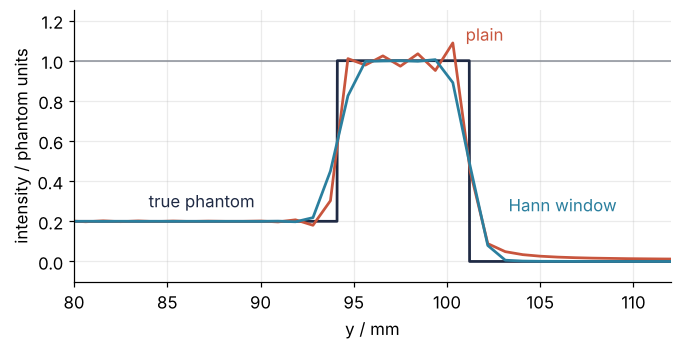
Window and zero-filling are the two knobs you will meet in scanner software, usually under those names.

Step 5: Skip every second line and watch the image fold

Keep every second line, as a scanner does when told to skip them, reconstruct on the grid that is left, and get both fields of view from the line spacing:

half = kspace[::2]                                # line 128 becomes line 64, still N/2, so recon applies
image_half = recon(half)
ky = np.fft.fftshift(np.fft.fftfreq(N, d=dx))     # sorted line positions / (1/mm)
print("k-space:", kspace.shape, "->", half.shape, "  image:", image_half.shape)
print(f"field of view in y: {1 / (ky[1] - ky[0]):.1f} mm -> {1 / (ky[2] - ky[0]):.1f} mm")

k-space: (256, 256) -> (128, 256)   image: (128, 256)
field of view in y: 240.0 mm -> 120.0 mm

In the prerequisite, a record of length \(T\) gave frequencies spaced by \(1/T\). Read with the two domains exchanged, lines spaced by \(\Delta k_y\) give an image that repeats every \(1/\Delta k_y\) in \(y\), so doubling the spacing halves the field of view to 120 mm.

The head does not fit. In the prerequisite, sampling a signal every \(\Delta t\) folded anything above \(1/(2\Delta t)\) back onto a false lower frequency. Sampling k-space every \(\Delta k_y\) folds anything beyond \(\pm 1/(2\Delta k_y) = \pm 60\) mm back into the image, so the top of the skull, near 100 mm in Step 4's profile, lands just below the center, and the bottom just above. This is fold-over.

It happens only vertically. Each line still has its 256 readout samples at the old spacing, so the image stays 240 mm wide. Skipping readout samples would save no time, which is why fold-over in MRI is always along the phase-encode direction.

Half the data also costs signal-to-noise. Measure the noise on the real part of the phase-corrected image, where it averages to zero, in the strip \(|x| > 100\) mm outside the head, not on the magnitude (Pitfall 2):

ramp = np.exp(-2j * np.pi * (2 / FOV) * x)
background = np.abs(x) > 100
sd_full = (image * ramp).real[:, background].std()
sd_half = (image_half * ramp).real[:, background].std()
print(f"background noise: 256 lines {sd_full:.4f}, 128 lines {sd_half:.4f}, ratio {sd_half / sd_full:.2f}")

background noise: 256 lines 0.0078, 128 lines 0.0108, ratio 1.39

ifft2 divides by the number of samples, so each pixel is an average over all of them, and an average over half as many samples with the same noise each is noisier by \(\sqrt2 \approx 1.41\). Measured: 1.39. The full image and the folded one, at the same scale:

Copy

fig, axes = plt.subplots(1, 2, figsize=(8, 4), sharey=True)
axes[0].imshow(np.abs(image), cmap="gray", vmin=0, vmax=0.5, origin="lower", extent=extent)
for y_edge in [-FOV / 4, FOV / 4]:
    axes[0].axhline(y_edge, color=SECOND, lw=1, ls="--")
axes[1].imshow(np.abs(image_half), cmap="gray", vmin=0, vmax=0.5, origin="lower",
               extent=[-FOV / 2, FOV / 2, -FOV / 4, FOV / 4])
for ax, label in zip(axes, ["256 lines", "128 lines"]):
    ax.text(0, 1.02, label, transform=ax.transAxes, va="bottom", color=INK)
    ax.set(xlabel="x / mm", xlim=(-FOV / 2, FOV / 2), ylim=(-FOV / 2, FOV / 2))
    ax.grid(False)
axes[0].set(ylabel="y / mm")
plt.show()

Pitfalls

Shifts that do not match the data. The symptom is either the head split into four quarters sitting in the corners of the image, or a magnitude that looks right with a phase that flips sign from pixel to pixel, a checkerboard \((-1)^{m+n}\) over the pixel indices \(m, n\). The cause is that the order of the data and the order the code assumes disagree. The quarters come from leaving out the final fftshift. The checkerboard comes from an ifftshift missing on centered data or applied to data already in NumPy's order: it is Step 3's shift theorem with a shift of \(N/2 = 128\) samples, whose phase ramp \(e^{i\pi m}\) changes sign at every pixel (for even \(N\)). The fix is Step 1's center test before anything else, then recon or the corner-data call at the end of Step 2. Never a bare ifft2.

Measuring noise on the magnitude image. The tempting shortcut takes the mean magnitude of a dark background region as the noise level. The magnitude is never negative, so noise that averages to zero in each channel does not average to zero there, and the signal-to-noise ratio comes out too low:

print(f"background: mean |image| = {np.abs(image[:, background]).mean():.4f}, "
      f"noise SD per channel = {sd_full:.4f}, ratio {np.abs(image[:, background]).mean() / sd_full:.2f}")

background: mean |image| = 0.0097, noise SD per channel = 0.0078, ratio 1.25

The mean of the magnitude is 25 % above the noise standard deviation it is taken for. Measure on the real part of the phase-corrected image, as Step 5 does, or in a region whose signal is many times the noise, where magnitude and real part agree.

Expecting software to undo fold-over. The ghost of the skull stays in the brain whatever filter you apply to the magnitude image. Step 5's folding adds two positions into one pixel, and a single image does not record which part came from where. The fix is in the acquisition: a field of view that covers the object in the phase-encode direction (scanners call the extra lines phase oversampling), the phase-encode direction along the short axis of the object, or several receive coils. Here they have to combine: the head is 202 mm tall and 152 mm wide, so turning the phase-encode direction to \(x\) still leaves 32 mm more than Step 5's 120 mm.

Variations

• Several receive coils. Each coil records its own k-space. Reconstruct each with recon and combine them as np.sqrt(np.sum(np.abs(images)**2, axis=0)). The differences between the coils are what parallel imaging, SENSE and GRAPPA, uses to unfold Step 5's ghost.
• A 3D acquisition. Two phase-encode directions and one readout. Use np.fft.ifftn and give both shifts the same axes=(0, 1, 2).
• Partial Fourier. Measure about 5/8 of the lines. For a real object \(F(-\mathbf k) = F^*(\mathbf k)\), which fills in much of the rest, once the phase of Step 3 has been estimated and removed.
• Radial or spiral sampling. The samples no longer sit on a grid, and ifft2 gives way to a nonuniform FFT, which interpolates them onto one first.

Cheat sheet

np.unravel_index(np.abs(k).argmax(), k.shape)   # center test: near (N/2, N/2) = sorted, near (0, 0) = NumPy order
np.fft.fftfreq(N, d=dx)                         # frequencies in NumPy order; fftshift sorts them
img = np.fft.fftshift(np.fft.ifft2(np.fft.ifftshift(k)))   # sorted (scanner) k-space; right for odd N too
img = np.fft.fftshift(np.fft.ifft2(k))          # k-space in NumPy order, zero at the corner
np.abs(img), np.angle(img)                      # look at the magnitude; the phase carries offsets
k[::R]                                          # every R-th line: field of view FOV / R along that axis
k * np.outer(np.hanning(N), np.hanning(N))      # Hann window: no ringing, softer edges
np.pad(k, N // 2)                               # zero-fill: smaller pixels, same resolution
np.fft.fftshift(np.fft.ifftn(np.fft.ifftshift(k, axes=a), axes=a), axes=a)   # 3D: a = (0, 1, 2)

Further reading

• numpy.fft, in particular "Implementation details" for the order of the frequencies, and the reference pages of fftshift and ifftshift.
• Nishimura, Principles of Magnetic Resonance Imaging, for k-space, sampling, and fold-over from the scanner's side; Brown, Cheng, Haacke, Thompson, Venkatesan, Magnetic Resonance Imaging: Physical Principles and Sequence Design (2nd ed., 2014), for the sequences behind the lines.
• Gach, Tanase, Boada, "2D & 3D Shepp-Logan phantom standards for MRI" (2008), for the phantom's k-space in closed form, and Toft, The Radon Transform: Theory and Implementation (1996), for the modified table.
• Related tutorials on this site: The Fourier transform: asking a signal how much of each frequency it contains, the prerequisite; Filtering with scipy.signal: mains hum and noise out of an ECG, windows in time; Counting cells with scipy.ndimage: how many are there, and how large?, what to do with an image next; Colormaps: why a rainbow scale draws features that are not in the data, why gray for magnitude and a cyclic map for phase. Planned: the same reconstruction in Julia with FFTW.jl.
• Download the notebook. It was executed with the library versions in the header.