Compute Christoffel symbols and the curvature of a metric with SymPy

The problem

You have a metric \(g_{ab}\) in coordinates \(x^a\) and want its Christoffel symbols, Riemann and Ricci tensors, and a curvature invariant, without the sign errors of working out 40 independent Christoffel symbols and 20 Riemann components by hand. The convention is Carroll's,

and the invariant is the Kretschmann scalar

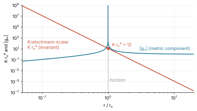
which the code sums in the equivalent form \(R^{ab}{}_{cd}R^{cd}{}_{ab}\) with \(R^{ab}{}_{cd} = g^{be}R^a{}_{ecd}\). The example is Schwarzschild, \(ds^2 = -(1 - r_s/r)\,dt^2 + dr^2/(1 - r_s/r) + r^2 d\theta^2 + r^2\sin^2\theta\, d\phi^2\), and the figure sets \(K\) beside the metric component \(|g_{rr}|\), because only one blows up at the horizon. New beyond SymPy from the ground up are sp.diag for a diagonal matrix, .inv() for its inverse, and sp.Matrix(n, n, f) for a matrix filled from a function of the indices. Swap in your own metric in the first section of the cell; the last is specific to Schwarzschild.

The code

Copy

import itertools
import numpy as np
import sympy as sp
import matplotlib.pyplot as plt

# ---- coordinates and metric: replace with your own
t, r, theta, phi = sp.symbols("t r theta phi")
r_s = sp.Symbol("r_s", positive=True)
x = [t, r, theta, phi]
f = 1 - r_s / r
g = sp.diag(-f, 1 / f, r**2, r**2 * sp.sin(theta)**2)      # sp.Matrix([[...], ...]) for off-diagonal terms
g_inv = sp.simplify(g.inv())
n = len(x)

# ---- Christoffel symbols (any metric)
# g[a, b] indexes a SymPy matrix, Gamma[a][b][c] nested lists; the first index is the upper one
Gamma = [[[sp.simplify(sum(g_inv[a, d] * (sp.diff(g[d, c], x[b]) + sp.diff(g[d, b], x[c])
                                          - sp.diff(g[b, c], x[d])) for d in range(n)) / 2)
           for c in range(n)] for b in range(n)] for a in range(n)]
nonzero = [(a, b, c) for a in range(n) for b in range(n) for c in range(b, n) if Gamma[a][b][c] != 0]
for a, b, c in nonzero:
    print(f"Gamma^{x[a]}_{x[b]}{x[c]} = {Gamma[a][b][c]}")
print(f"{len(nonzero)} of {n**2 * (n + 1) // 2} independent Christoffel symbols are nonzero")

# ---- Riemann, Ricci, Kretschmann (any metric)
# R[a][b][c][d] is R^a_bcd
R = [[[[sp.simplify(sp.diff(Gamma[a][d][b], x[c]) - sp.diff(Gamma[a][c][b], x[d])
                    + sum(Gamma[a][c][e] * Gamma[e][d][b] - Gamma[a][d][e] * Gamma[e][c][b] for e in range(n)))
        for d in range(n)] for c in range(n)] for b in range(n)] for a in range(n)]
Ric = sp.Matrix(n, n, lambda b, d: sp.simplify(sum(R[a][b][a][d] for a in range(n))))
# M[a][b][c][d] is R^ab_cd, the second index raised
M = [[[[sum(g_inv[b, e] * R[a][e][c][d] for e in range(n)) for d in range(n)] for c in range(n)]
      for b in range(n)] for a in range(n)]
K = sp.simplify(sum(M[a][b][c][d] * M[c][d][a][b]
                    for a, b, c, d in itertools.product(range(n), repeat=4)))   # all index tuples (a, b, c, d)
print("Ricci tensor is zero:", Ric == sp.zeros(n))
print("Kretschmann scalar K =", K)

# ---- Schwarzschild check and plot: replace or delete for your own metric
print("K r_s^4 at the horizon r = r_s:", sp.simplify(K.subs(r, r_s) * r_s**4))
K_np = sp.lambdify((r, r_s), K, "numpy")
g_rr_np = sp.lambdify((r, r_s), g[1, 1], "numpy")
rho_in = 1 - np.geomspace(0.95, 1e-10, 300)                 # r / r_s inside the horizon, crowding toward it
rho_out = 1 + np.geomspace(1e-10, 19, 300)                  # and outside

fig, ax = plt.subplots(figsize=(7, 3.6), dpi=110)
ax.plot(np.concatenate([rho_in, rho_out]), K_np(np.concatenate([rho_in, rho_out]), 1.0), color="#c8553d", lw=1.8)
for side in (rho_in, rho_out):                              # two pieces, so no line jumps across r = r_s
    ax.plot(side, np.abs(g_rr_np(side, 1.0)), color="#2a7f9e", lw=1.8)
ax.axvline(1, color="#8a8f98", ls="--", lw=1)
ax.plot(1, 12, "o", color="#c8553d", ms=6)
ax.text(1.15, 30, "K rₛ⁴ = 12", color="#c8553d")
ax.text(0.06, 10, "Kretschmann scalar\nK rₛ⁴ (invariant)", color="#c8553d")
ax.text(3, 4, "|gᵣᵣ| (metric component)", color="#2a7f9e", va="bottom")
ax.text(1.06, 1e-5, "horizon", color="#8a8f98")
ax.set(xscale="log", yscale="log", xlim=(0.05, 20), ylim=(1e-7, 1e9), xlabel="r / rₛ", ylabel="K rₛ⁴ and |gᵣᵣ|")
ax.spines[["top", "right"]].set_visible(False)
ax.grid(alpha=0.25)
plt.show()

Gamma^t_tr = r_s/(2*r*(r - r_s))
Gamma^r_tt = r_s*(r - r_s)/(2*r**3)
Gamma^r_rr = -r_s/(2*r*(r - r_s))
Gamma^r_thetatheta = -r + r_s
Gamma^r_phiphi = (-r + r_s)*sin(theta)**2
Gamma^theta_rtheta = 1/r
Gamma^theta_phiphi = -sin(2*theta)/2
Gamma^phi_rphi = 1/r
Gamma^phi_thetaphi = 1/tan(theta)
9 of 40 independent Christoffel symbols are nonzero
Ricci tensor is zero: True
Kretschmann scalar K = 12*r_s**2/r**6
K r_s^4 at the horizon r = r_s: 12

The knobs

The input is any symmetric sp.Matrix in any number of dimensions: n = len(x) carries through the two middle sections, and only the first and the last change. On the 2-sphere of radius \(a\), two coordinates and sp.diag(a**2, a**2*sp.sin(theta)**2), the same two sections return \(K = 4/a^4\) and a Ricci tensor equal to \(g_{ab}/a^2\), which is not zero. The simplifier is the other knob. simplify tries a list of rewrites and keeps the shortest result, a heuristic, and no simplifier can be complete (see Computer algebra: formulas as trees). That is why the output says -sin(2*theta)/2 and 1/tan(theta) where Carroll writes \(-\sin\theta\cos\theta\) and \(\cot\theta\); trigsimp leaves both as they are. When you know which rewrite an expression needs, factor or cancel gets there faster and more predictably. cancel puts an expression over one common denominator and divides out the factors that numerator and denominator share; for a metric with many off-diagonal terms, Kerr for instance, it is the first thing to try per component. It treats \(\sin\theta\) and \(\cos\theta\) as unrelated symbols, though, so run trigsimp or simplify on what is left before you compare it with zero. Books with the opposite sign convention for \(R^a{}_{bcd}\) flip the sign of Riemann and Ricci but not of \(K\), which is quadratic in Riemann. To switch, negate the whole Riemann expression, all four terms. Negating only the two derivative terms gives something that is not a tensor, and its Ricci tensor on Schwarzschild is not zero.

True for the Ricci tensor is the vacuum Einstein equation, \(R_{ab} = 0\), and nothing more. It does not say the spacetime is flat: \(K\) is not zero, so neither is Riemann. At the horizon \(K = 12/r_s^4\), finite, while \(g_{rr}\) diverges there, so that divergence belongs to the coordinates and a better choice of them removes it. At \(r = 0\) the invariant itself diverges, and no change of coordinates removes that. The same metric's light rays are traced in Ray tracing a black hole with solve_ivp. SymPy has a module for all of this, sympy.diffgeom, with coordinate-system and form objects; the explicit loops are kept here because each line reads like one of the formulas above.

Pitfalls

Simplifying too late. Leave out the sp.simplify around the Christoffel symbols and the Riemann components, and the finished sum for \(K\) is a fraction you cannot read:

G_late = [[[sum(g_inv[a, d] * (sp.diff(g[d, c], x[b]) + sp.diff(g[d, b], x[c]) - sp.diff(g[b, c], x[d]))
                for d in range(n)) / 2 for c in range(n)] for b in range(n)] for a in range(n)]
R_late = [[[[sp.diff(G_late[a][d][b], x[c]) - sp.diff(G_late[a][c][b], x[d])
             + sum(G_late[a][c][e] * G_late[e][d][b] - G_late[a][d][e] * G_late[e][c][b] for e in range(n))
             for d in range(n)] for c in range(n)] for b in range(n)] for a in range(n)]
M_late = [[[[sum(g_inv[b, e] * R_late[a][e][c][d] for e in range(n)) for d in range(n)] for c in range(n)]
           for b in range(n)] for a in range(n)]
K_late = sum(M_late[a][b][c][d] * M_late[c][d][a][b] for a, b, c, d in itertools.product(range(n), repeat=4))
print(f"operations in K: {sp.count_ops(K_late)} unsimplified, {sp.count_ops(K)} simplified")

operations in K: 317 unsimplified, 4 simplified

That is 317 operations where the simplified \(K\) has 4. On Schwarzschild one simplify at the end still gets back to 12*r_s**2/r**6 in under a second. Every contraction multiplies sums by sums, though, so the swell compounds with each step and with each off-diagonal entry of the metric, and the expression that last simplify faces grows with it. Simplify g_inv once and every component once, when it is made, as the cell does; each later step then starts from short expressions.

Indices in the wrong place. Wrong signs or wrong powers of \(1 - r_s/r\) in \(\Gamma\) or \(K\) almost always come from g where g_inv belongs, or from contracting Ricci on the wrong pair of indices. Keep the upper index first, as the comments in the cell say, and test any change on Schwarzschild first, where the Ricci tensor must vanish and \(K\) must be \(12 r_s^2/r^6\).

A zero that does not compare equal. Ric == sp.zeros(n) prints False for a metric that is a vacuum solution. == compares the form of two expressions, not their value, and a sum of simplified Riemann components can still be a zero written as two fractions:

Ric_late = sp.Matrix(n, n, lambda b, d: sum(R[a][b][a][d] for a in range(n)))   # no sp.simplify
print(Ric_late == sp.zeros(n), "  R_tt =", Ric_late[0, 0])

False   R_tt = r_s*(-r + r_s)/r**4 + r_s*(r - r_s)/r**4

The entry is \(r_s(r_s - r)/r^4 + r_s(r - r_s)/r^4\), zero to anyone who reads it and False to ==. Here simplifying is about the comparison, not the size, so do it right before you compare: the cell simplifies each Ricci entry as it builds the matrix, and on a matrix you already have, Ric.applyfunc(sp.simplify) == sp.zeros(n) does the same.