Computer algebra: formulas as trees, exact until you ask for digits (Python)

The question

Ask Python for 0.1 · 3 − 0.3 and NumPy for the square root of 8, then ask SymPy, Python's computer algebra system, for the same two things with exact fractions:

Show code

import sympy as sp
import numpy as np
import matplotlib.pyplot as plt
from scipy.special import ellipk

plt.rcParams.update({
    "figure.figsize": (7, 3.6), "figure.dpi": 110,
    "axes.spines.top": False, "axes.spines.right": False,
    "axes.grid": True, "grid.alpha": 0.25,
    "font.size": 11, "lines.linewidth": 1.8,
})
INK, ACCENT, SECOND, MUTED = "#1f2a44", "#c8553d", "#2a7f9e", "#8a8f98"

print(f"float64  0.1 * 3 - 0.3                          = {0.1 * 3 - 0.3!r}")
print(f"SymPy    Rational(1, 10) * 3 - Rational(3, 10)  = {sp.Rational(1, 10) * 3 - sp.Rational(3, 10)}")
print(f"float64  np.sqrt(8)                             = {float(np.sqrt(8))!r}")
print(f"SymPy    sp.sqrt(8)                             = {sp.sqrt(8)}")

float64  0.1 * 3 - 0.3                          = 5.551115123125783e-17
SymPy    Rational(1, 10) * 3 - Rational(3, 10)  = 0
float64  np.sqrt(8)                             = 2.8284271247461903
SymPy    sp.sqrt(8)                             = 2*sqrt(2)

The float result is 5.55 × 10⁻¹⁷ instead of 0, because 0.1 has no exact binary form; Floating-point numbers: why 0.1 + 0.2 is not 0.3, and a derivative's best step takes that apart. SymPy gets 0, and for √8 it does not give a number at all: it answers 2*sqrt(2) where NumPy prints 2.8284271247461903.

The same contrast decides a physical number. A pendulum released at amplitude θ₀ swings with a period T longer than its small-angle period T₀, by

\[\frac{T}{T_0} - 1 = \frac{2}{\pi}\,K\!\left(\sin^2\frac{\theta_0}{2}\right) - 1, \qquad K(m) = \int_0^{\pi/2} \frac{d\varphi}{\sqrt{1 - m\sin^2\varphi}} ,\]

where \(K\) is the complete elliptic integral of the first kind, written with the parameter \(m\) as both scipy.special.ellipk and sympy.elliptic_k write it (some textbooks use \(k = \sqrt{m}\) instead). The formula follows from energy conservation, and SymPy from the ground up: where the pendulum's 1.74 % comes from derives it. Here it is enough that SciPy and SymPy both evaluate \(K\). This is the correction from 10⁻⁹ rad to 90°, computed three ways from the same 200 amplitudes: the formula in float64 with SciPy, its first series term θ₀²/16, and the formula in SymPy.

Show code

theta0 = sp.Symbol("theta0")
ratio = 2 * sp.elliptic_k(sp.sin(theta0 / 2) ** 2) / sp.pi      # T/T0, kept as an expression
corr = ratio - 1                                                # the subtraction stays inside it


def float_corr(a):
    return 2 / np.pi * ellipk(np.sin(a / 2) ** 2) - 1


def sympy_corr(a):
    # sp.Rational(a) is the exact value of the float a, so both methods get the same input
    return float(corr.subs(theta0, sp.Rational(a)).evalf(16))


a = np.logspace(-9, np.log10(np.pi / 2), 200)                   # amplitudes / rad
c_float = float_corr(a)
c_exact = np.array([sympy_corr(x) for x in a])
c_term = a**2 / 16

print("theta0          float64     first term       SymPy")
for x, name in [(1e-8, "1e-8 rad"), (1e-7, "1e-7 rad"), (1e-6, "1e-6 rad"), (np.pi / 6, "30°")]:
    print(f"{name:9s}  {float_corr(x):11.3e}  {x**2 / 16:11.3e}  {sympy_corr(x):11.3e}")

floor = 1e-21                                                   # where the zeros of float64 are drawn
pos = c_float > 0
fig1, (ax, bx) = plt.subplots(2, 1, figsize=(7, 4.6), sharex=True)
ax.plot(a, c_exact, color=INK)
ax.plot(a, c_term, color=SECOND, lw=1.2, ls=(0, (5, 2)))
ax.plot(a[pos], c_float[pos], color=ACCENT, lw=1.2)
ax.plot(a[~pos], np.full((~pos).sum(), floor), "o", ms=4, color=ACCENT)
ax.text(6e-8, floor, "float64 gives 0", color=ACCENT, va="center")
ax.text(1e-5, 1e-14, "all three agree", color=INK)
ax.set(xscale="log", yscale="log", ylim=(floor / 20, 1), yticks=[1e-20, 1e-15, 1e-10, 1e-5, 1],
       ylabel="T/T₀ − 1")

# the same curves divided by the SymPy one: 1 means they agree
bx.axhline(1, color=INK, lw=1.8, zorder=3)
bx.plot(a, c_term / c_exact, color=SECOND, lw=1.2, ls=(0, (5, 2)))
bx.plot(a, c_float / c_exact, "o", ms=2.5, color=ACCENT)
bx.axvline(np.pi / 6, color=MUTED, lw=1, ls="--")
bx.text(np.pi / 6 / 1.2, 0.83, f"30°: θ₀²/16 gives {100 * (np.pi / 6)**2 / 16:.3f} %,\nSymPy {100 * sympy_corr(np.pi / 6):.3f} %",
        ha="right", va="bottom", color=SECOND)
bx.text(1.5e-6, 1.08, "float64 scatters", color=ACCENT, va="bottom")
bx.text(1.2e-9, 0.82, "float64 is 0", color=ACCENT, va="bottom")
bx.set(xscale="log", xlim=(1e-9, np.pi / 2), ylim=(0.8, 1.2),
       xlabel="θ₀ / rad", ylabel="result / SymPy")
plt.show()

theta0          float64     first term       SymPy
1e-8 rad     0.000e+00    6.250e-18    6.250e-18
1e-7 rad     6.661e-16    6.250e-16    6.250e-16
1e-6 rad     6.239e-14    6.250e-14    6.250e-14
30°          1.741e-02    1.713e-02    1.741e-02

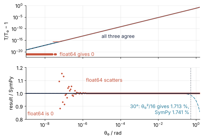
Top: pendulum period correction T/T₀ − 1 against amplitude θ₀ in rad, log-log; float64 gives 0 below 2.5e-8 rad. Bottom: each result divided by the SymPy value; float64 scatters below 1e-6 rad, the first term θ₀²/16 falls away at large amplitude, 1.713 % against 1.741 % at 30°.

Two different errors are in the picture. At small amplitudes, on the left of both panels, the float64 result starts to scatter below 10⁻⁶ rad. At 10⁻⁷ rad it reads 6.66 × 10⁻¹⁶ against 6.25 × 10⁻¹⁶, 7 % off, and below 2.5 × 10⁻⁸ rad it is exactly 0. At 10⁻⁸ rad the ratio T/T₀ is 1.00000000000000000625, and a float, which keeps about 16 digits, stores it as 1. That is rounding. At large amplitudes the first term falls away from the SymPy value and gives 1.713 % at 30° against 1.741 %, because the series was cut after one term. That is truncation.

SymPy's curve is right at both ends, from the same float inputs and with the same 16 digits asked for, all of them correct. What does it store instead of digits, and how does that get both ends right?

The idea: a formula is a tree, and calculus is rules on trees

A computer algebra system never computes θ₀ cos(ωt). It stores it as a tree: each inner node is an operation, a product or a cosine, and the leaves are symbols and exact numbers. SymPy's srepr prints the tree as it is stored:

Show code

omega, t = sp.symbols("omega t")
expr = theta0 * sp.cos(omega * t)
print(sp.srepr(expr))

Mul(Symbol('theta0'), cos(Mul(Symbol('omega'), Symbol('t'))))

Read it from the outside in: a product, Mul, of the symbol θ₀ and a cosine, whose argument is another product, of ω and t. Every operation on the expression rewrites this tree into another tree by rules. At no point does a number with digits appear.

Differentiation shows it best. diff(expr, t) starts at the root, applies the rule for the node it is on, and calls itself on the children the rule asks for. The table it needs is short, base cases first:

Leaves. dt/dt = 1. Any other symbol, θ₀ or ω, and any number give 0. That is the whole of how the system knows θ₀ is constant: it is a symbol other than t.
Products. d(uv) = du · v + u · dv, which sends the walk into both factors.
Cosine, with the chain rule. d cos u = −sin u · du, where du sends the walk one level down.

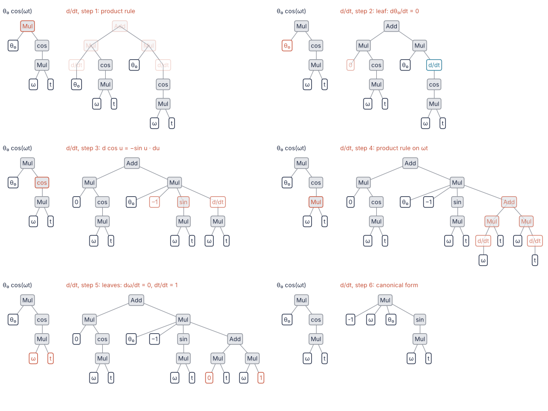
On θ₀ cos(ωt) the walk goes like this. The product rule at the root splits it into two terms. In the first, the θ₀ leaf gives 0, so that term drops. In the second, the cosine rule gives −sin(ωt) times d(ωt)/dt, and the product rule on ωt meets the ω leaf, which gives 0, and the t leaf, which gives 1, so d(ωt)/dt = ω. The recursion stops because every path has ended at a leaf. Here are three stages of the walk:

Show code

NAMES = {"theta0": "θ₀", "omega": "ω", "t": "t"}


def tree(e):
    """A SymPy expression as nested (label, kind, children) tuples, read off func and args."""
    if not e.args:
        return (NAMES.get(str(e), str(e).replace("-", "−")), "leaf", [])
    return (e.func.__name__, "op", [tree(c) for c in e.args])


def node(label, *children, kind=None):
    """A hand-listed node, for the stage SymPy never stores."""
    return (label, kind or ("op" if children else "leaf"), list(children))


def layout(n, depth=0, x=None, out=None):
    """Leaves side by side, two-character labels a little wider; each parent above the middle of its children."""
    x = [0] if x is None else x
    label, kind, children = n
    if children:
        xs = [layout(c, depth + 1, x, out) for c in children]
        pos = (xs[0] + xs[-1]) / 2
    else:
        w = 1.0 if len(label) == 1 else 1.35
        xs, pos = [], x[0] + w / 2
        x[0] += w
    out.append((pos, -depth, label, kind, xs))
    return pos


STYLE = {"leaf": dict(fc="white", ec=INK, color=INK),
         "op": dict(fc="#e4e6ea", ec=MUTED, color=INK),
         "new": dict(fc="white", ec=ACCENT, color=ACCENT),        # what a rule just produced
         "pending": dict(fc="white", ec=SECOND, color=SECOND),    # a derivative still to take
         "dead": dict(fc="white", ec=MUTED, color=MUTED)}         # a term that is already 0


def draw_tree(ax, nodes, formula, depth):
    for xp, yp, label, kind, xs in nodes:
        for xc in xs:
            ax.plot([xp, xc], [yp, yp - 1], color=MUTED, lw=1, zorder=1)
    for xp, yp, label, kind, xs in nodes:
        style = dict(STYLE[kind])
        color = style.pop("color")
        ax.text(xp, yp, label, ha="center", va="center", color=color, zorder=2,
                bbox=dict(boxstyle="round,pad=0.3", lw=1.2, **style))
    xs_all = [p[0] for p in nodes]
    ax.text((min(xs_all) + max(xs_all)) / 2, -depth - 0.9, formula, ha="center", va="center", color=INK)
    ax.set(xlim=(min(xs_all) - 0.6, max(xs_all) + 0.6), ylim=(-depth - 1.3, 0.4))
    ax.set_axis_off()


omega_t = node("Mul", node("ω"), node("t"))
middle = node("Add",
              node("Mul", node("0", kind="new"), node("cos", omega_t), kind="dead"),
              node("Mul", node("θ₀"), node("−1"), node("sin", omega_t), node("d/dt", omega_t, kind="pending")))
dexpr = sp.diff(expr, t)

stages = [(tree(expr), "θ₀ cos(ωt)"),
          (middle, "0·cos(ωt) + θ₀·(−1)·sin(ωt)·d(ωt)/dt"),
          (tree(dexpr), "−ωθ₀ sin(ωt)")]
laid = []
for n, formula in stages:
    nodes = []
    layout(n, out=nodes)
    laid.append((nodes, formula))
depth = max(-p[1] for nodes, _ in laid for p in nodes)
spans = [max(p[0] for p in nodes) - min(p[0] for p in nodes) + 1.2 for nodes, _ in laid]
fig2, axes = plt.subplots(1, 3, figsize=(8, 3.3), gridspec_kw=dict(width_ratios=spans, wspace=0.08))
for ax, (nodes, formula) in zip(axes, laid):
    draw_tree(ax, nodes, formula, depth)
plt.show()

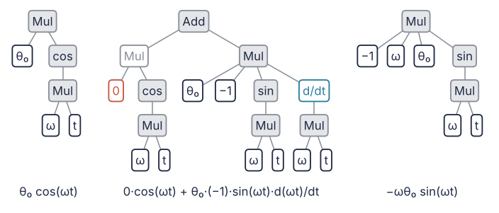
Expression tree of θ₀ cos(ωt) differentiated in t, in three stages: the original tree; after the product and cosine rules, with the θ₀ term at zero and d(ωt)/dt still pending; the final tree of −θ₀ω sin(ωt) with −1 as its own leaf.

The outer trees are SymPy's own, read off func and args. The middle one is a stage of the walk that SymPy never stores, listed by hand from the rules: the θ₀ term with its 0 on the left, and on the right the one node, d(ωt)/dt, still waiting for the walk to reach its leaves. The animation does the same walk one rule at a time:

Animation of SymPy's differentiation of θ₀ cos(ωt): the walk visits each node of the tree, applies one rule per step, and stops at the leaves; the derivative tree −θ₀ω sin(ωt) grows beside it.

Show code

"""Derivative tree: SymPy's differentiation of theta0*cos(omega*t) in t, one rule per step.

Renders ../../assets/derivative-tree.gif for the computer algebra tutorial. Left: the tree of
the expression, with the node the walk is on in red. Right: the derivative as a tree, growing
as the rules are applied; new nodes fade in red and settle to ink. The last stage is the tree
SymPy returns, read off its func and args. Run it from any directory:

    python scene.py
"""
from pathlib import Path

import sympy as sp
import matplotlib.pyplot as plt
from matplotlib.animation import FuncAnimation, PillowWriter

OUT = Path(__file__).resolve().parents[2] / "assets" / "derivative-tree.gif"
INK, ACCENT, SECOND, MUTED = "#1f2a44", "#c8553d", "#2a7f9e", "#8a8f98"
plt.rcParams.update({"font.size": 11})

NAMES = {"theta0": "θ₀", "omega": "ω", "t": "t"}


def N(label, *children, key=None):
    """A node: label, children, and a key that says which stage created it."""
    return dict(label=label, children=list(children), key=key)


def from_expr(e, key=None):
    if not e.args:
        return N(NAMES.get(str(e), str(e)), key=key)
    return N(e.func.__name__, *[from_expr(c, key) for c in e.args], key=key)


def layout(n, depth=0, x=None, out=None):
    x = [0] if x is None else x
    if n["children"]:
        xs = [layout(c, depth + 1, x, out) for c in n["children"]]
        pos = (xs[0] + xs[-1]) / 2
    else:
        w = 1.0 if len(n["label"]) == 1 else 1.35                  # two-character leaves a little wider
        xs, pos = [], x[0] + w / 2
        x[0] += w
    out.append(dict(x=pos, y=-depth, node=n, xs=xs))
    return pos


# ---- the expression and the stages of the walk
theta0, omega, t = sp.symbols("theta0 omega t")
expr = theta0 * sp.cos(omega * t)
source = from_expr(expr)
root, th_leaf, cos_node = source, source["children"][0], source["children"][1]
wt = cos_node["children"][0]
w_leaf, t_leaf = wt["children"]


def wt_tree(key=None):
    return N("Mul", N("ω", key=key), N("t", key=key), key=key)


def pending(of, key):
    return N("d/dt", of, key=key)


stages = [  # (rule title, source nodes visited, derivative tree)
    ("product rule", [root],
     N("Add", N("Mul", pending(N("θ₀"), 1), N("cos", wt_tree()), key=1),
       N("Mul", N("θ₀"), pending(N("cos", wt_tree()), 1), key=1), key=1)),
    ("leaf: dθ₀/dt = 0", [th_leaf],
     N("Add", N("Mul", N("0", key=2), N("cos", wt_tree())),
       N("Mul", N("θ₀"), pending(N("cos", wt_tree()), None)))),
    ("d cos u = −sin u · du", [cos_node],
     N("Add", N("Mul", N("0"), N("cos", wt_tree())),
       N("Mul", N("θ₀"), N("−1", key=3), N("sin", wt_tree(), key=3), pending(wt_tree(), 3)))),
    ("product rule on ωt", [wt],
     N("Add", N("Mul", N("0"), N("cos", wt_tree())),
       N("Mul", N("θ₀"), N("−1"), N("sin", wt_tree()),
         N("Add", N("Mul", pending(N("ω"), 4), N("t"), key=4),
           N("Mul", N("ω"), pending(N("t"), 4), key=4), key=4)))),
    ("leaves: dω/dt = 0, dt/dt = 1", [w_leaf, t_leaf],
     N("Add", N("Mul", N("0"), N("cos", wt_tree())),
       N("Mul", N("θ₀"), N("−1"), N("sin", wt_tree()),
         N("Add", N("Mul", N("0", key=5), N("t")), N("Mul", N("ω"), N("1", key=5)))))),
    ("canonical form", [], from_expr(sp.diff(expr, t), key=6)),
]

PER_STAGE, HOLD = 16, 20
frames = len(stages) * PER_STAGE + HOLD


def laid(tree):
    nodes = []
    layout(tree, out=nodes)
    return nodes


# fixed limits for every frame, so that the trees do not zoom between stages
all_right = [laid(d) for _, _, d in stages]
span_r = max(max(p["x"] for p in ns) - min(p["x"] for p in ns) for ns in all_right)
depth_r = max(-p["y"] for ns in all_right for p in ns)
nodes_l = laid(source)
span_l = max(p["x"] for p in nodes_l) - min(p["x"] for p in nodes_l)

fig, (axl, axr) = plt.subplots(1, 2, figsize=(7, 3.5), dpi=80,
                               gridspec_kw=dict(width_ratios=[span_l + 1.2, span_r + 1.2]))
fig.subplots_adjust(left=0.01, right=0.99, top=0.88, bottom=0.03, wspace=0.04)


def draw(ax, tree, span, depth, highlight=(), new_key=None, age=0):
    ax.clear()
    ax.set_axis_off()
    nodes = laid(tree)
    shift = -min(p["x"] for p in nodes)          # left-aligned: the finished 0 term stays put while the rest grows
    for p in nodes:
        for xc in p["xs"]:
            ax.plot([p["x"] + shift, xc + shift], [p["y"], p["y"] - 1], color=MUTED, lw=1, zorder=1)
    for p in nodes:
        n = p["node"]
        op = bool(n["children"])
        color, ec, fc, alpha = INK, (MUTED if op else INK), ("#e4e6ea" if op else "white"), 1.0
        if n["label"] == "d/dt":                                   # a derivative still to take
            ec, color, fc = SECOND, SECOND, "white"
        if any(n is h for h in highlight):                         # the node the walk is on
            ec, color = ACCENT, ACCENT
        if new_key is not None and n["key"] == new_key and age < 10:   # what the rule just produced
            ec, color = ACCENT, ACCENT
            alpha = min(1.0, (age + 1) / 4)
        ax.text(p["x"] + shift, p["y"], n["label"], ha="center", va="center", color=color, alpha=alpha,
                fontsize=11, zorder=2, bbox=dict(boxstyle="round,pad=0.3", lw=1.2, fc=fc, ec=ec, alpha=alpha))
    ax.set(xlim=(-0.6, span + 0.6), ylim=(-depth - 0.5, 0.5))


def update(i):
    s = min(i // PER_STAGE, len(stages) - 1)
    age = i - s * PER_STAGE
    title, visited, deriv = stages[s]
    draw(axl, source, span_l, depth_r, highlight=visited)
    draw(axr, deriv, span_r, depth_r, new_key=s + 1, age=age)
    axl.set_title("θ₀ cos(ωt)", loc="left", fontsize=11, color=INK)
    axr.set_title(f"d/dt, step {s + 1}: {title}", loc="left", fontsize=11, color=ACCENT)
    return []


anim = FuncAnimation(fig, update, frames=frames, interval=1000 / 12)
OUT.parent.mkdir(parents=True, exist_ok=True)
anim.save(OUT, writer=PillowWriter(fps=12))
print(f"wrote {OUT} ({OUT.stat().st_size / 1e6:.2f} MB, {frames} frames)")

What SymPy returns is the angular velocity of a pendulum swinging as θ₀ cos(ωt):

Show code

print(dexpr)
print(sp.srepr(dexpr))

-omega*theta0*sin(omega*t)
Mul(Integer(-1), Symbol('omega'), Symbol('theta0'), sin(Mul(Symbol('omega'), Symbol('t'))))

The −1 is a leaf of its own, and the factors stand in SymPy's order, ω before θ₀, not in the order the rules produced them. The 0 and the 1 from the leaves are gone as well. SymPy puts every product into one canonical form as it builds it, which the formalization comes back to.

Exact numbers at the leaves

The leaves are also where the 0 in the first cell came from. Rational(1, 10) is not a binary approximation of a tenth, it is the pair of integers 1 and 10, and sqrt(8) is a small tree of its own:

Show code

print(sp.srepr(sp.Rational(1, 10)))
print(sp.srepr(sp.sqrt(8)))
print(sp.sqrt(2).evalf(50))

Rational(1, 10)
Mul(Integer(2), Pow(Integer(2), Rational(1, 2)))
1.4142135623730950488016887242096980785696718753769

Three times one tenth minus three tenths is then arithmetic on integer numerators and denominators, and it comes out 0 with nothing to round. √8 is stored as 2 times 2 to the power 1/2: SymPy pulled out the square factor and kept the rest as a power with a rational exponent, which is a statement about the number and not an approximation of it. Digits appear only when you ask for them with evalf(n), and then as many as you ask for, here 50 of √2.

evalf can do that because it does not compute in float64. It uses arbitrary-precision arithmetic from mpmath, the library under SymPy's numerics: floating-point numbers with as many digits as you set, 50 or 500, where float64 always has about 16. And evalf(n) promises n correct digits of the expression it is called on as a whole, not of each piece. To keep that promise it computes the pieces with more digits than n, its working precision, and raises that precision until the result has n right.

Formalization

An expression is a tree whose inner nodes are operations, each with an ordered tuple of children, and whose leaves are symbols or exact numbers. In SymPy the operation of a node is expr.func and its children are expr.args, and expr.func(*expr.args) rebuilds the node. Every algorithm in the system, from diff to series, takes such a tree apart and builds another one. Three consequences follow, and you meet each of them the first week you use a computer algebra system.

Show code

x, y = sp.symbols("x y")
print(f"x - y   ->  {sp.srepr(x - y)}")
print(f"x / y   ->  {sp.srepr(x / y)}")
print(f"x + x   ->  {x + x}")
print(f"(x + 1)**20 expanded:  {len(sp.expand((x + 1)**20).args)} terms")
print(f"x**20 - 1 factored:    {len(sp.factor_list(x**20 - 1)[1])} factors, {sp.factor(x**20 - 1)}")
print(f"simplify(sin(x)**2 + cos(x)**2) = {sp.simplify(sp.sin(x)**2 + sp.cos(x)**2)}")
for n in [4, 6]:
    M = sp.Matrix(n, n, lambda i, j: sp.Symbol(f"a{i}{j}"))
    print(f"determinant of a symbolic {n} x {n} matrix: {len(sp.expand(M.det(method='berkowitz')).args)} terms")

x - y   ->  Add(Symbol('x'), Mul(Integer(-1), Symbol('y')))
x / y   ->  Mul(Symbol('x'), Pow(Symbol('y'), Integer(-1)))
x + x   ->  2*x
(x + 1)**20 expanded:  21 terms
x**20 - 1 factored:    6 factors, (x - 1)*(x + 1)*(x**2 + 1)*(x**4 - x**3 + x**2 - x + 1)*(x**4 + x**3 + x**2 + x + 1)*(x**8 - x**6 + x**4 - x**2 + 1)
simplify(sin(x)**2 + cos(x)**2) = 1
determinant of a symbolic 4 x 4 matrix: 24 terms
determinant of a symbolic 6 x 6 matrix: 720 terms

There is no subtraction and no division. x − y is Add(x, Mul(-1, y)) and x/y is Mul(x, Pow(y, -1)): a difference is a sum with a factor −1, a quotient a product with a power −1. And x + x is 2*x the moment it is built, before you call anything. This is automatic simplification into one canonical form: terms are collected and arguments sorted, so that two expressions that differ only in order or in collected terms become the same tree and compare equal. The derivative above was built in that form.

Simplification has no single answer. expand and factor go in opposite directions, and which result is simpler depends on what you want to do next. (x + 1)²⁰ is one power, and expanded it is a sum of 21 terms. x²⁰ − 1 is two terms, and factored it is a product of six factors. simplify tries several such rewrites and keeps the shortest, which is a heuristic and not a method guaranteed to succeed. It is also how a system tests whether A = B: it simplifies A − B and looks for 0, and behind that test sits a theorem. Daniel Richardson proved in 1968 that whether an expression is zero is undecidable, for expressions built from x, π, ln 2, and the rational numbers with sums, products, and composition with exp, sin, and the absolute value. Undecidable means that no algorithm that always answers can exist, which is a stronger statement than that nobody has found one. So SymPy proves sin²x + cos²x = 1, and it cannot promise to recognize every zero you hand it.

Exact arithmetic has a price. Integers in SymPy have no size limit and rationals are never rounded, so results grow instead of being cut to 16 digits. The determinant of a general n × n matrix of symbols has n! terms, 24 at n = 4 and 720 at n = 6, and SymPy writes out every one. A float costs the same per number however large the computation gets. An exact computation pays twice: the terms multiply, as in the determinant, and each rational in them carries more digits as it goes. This is called expression swell, and it is why nobody runs a large simulation in a computer algebra system.

See it in code

Back to the pendulum, and to the answer. The cell prints the tree of the correction T/T₀ − 1, to show where the subtraction sits, and the series of T/T₀, to show where θ₀²/16 comes from. Then it evaluates the correction three ways at θ₀ = 10⁻⁸ rad and once more at 30°:

Show code

print("tree of T/T0 - 1:", sp.srepr(corr))
print("series of T/T0:  ", sp.series(ratio, theta0, 0, 6))

q = sp.Rational(1, 10**8)
print("\nat θ0 = 1e-8 rad")
print("  ratio.evalf(16) - 1   ", ratio.subs(theta0, q).evalf(16) - 1)
print("  (ratio - 1).evalf(16) ", corr.subs(theta0, q).evalf(16))
print("  (θ0**2 / 16).evalf(16)", (q**2 / 16).evalf(16))
p = sp.pi / 6
print(f"\nat 30°: SymPy {100 * float(corr.subs(theta0, p).evalf(16)):.3f} %, first term {100 * float((p**2 / 16).evalf(16)):.3f} %")

tree of T/T0 - 1: Add(Mul(Integer(2), Pow(pi, Integer(-1)), elliptic_k(Pow(sin(Mul(Rational(1, 2), Symbol('theta0'))), Integer(2)))), Integer(-1))
series of T/T0:   1 + theta0**2/16 + 11*theta0**4/3072 + O(theta0**6)

at θ0 = 1e-8 rad
  ratio.evalf(16) - 1    0
  (ratio - 1).evalf(16)  6.250000000000000e-18
  (θ0**2 / 16).evalf(16) 6.250000000000000e-18

at 30°: SymPy 1.741 %, first term 1.713 %

The root of the tree is an Add with Integer(-1) as one child, next to the Mul that holds 2/π and elliptic_k: the subtraction of 1 is a node of the formula, not a step already taken. The series is where the dashed curve of the first figure comes from: after the 1, its first term is θ₀²/16, and 11θ₀⁴/3072 is the next.

The three lines at 10⁻⁸ rad answer the question. Taking 16 digits of the ratio and then subtracting 1 gives 0, as float64 did: an exact formula does not help once its digits are taken before the subtraction. Asking evalf for 16 digits of the correction itself gives 6.250000000000000e-18. The subtraction is part of that expression, so evalf sees the cancellation. It raises its working precision until 16 digits of the difference are right. The series term θ₀²/16 gives the same number with no extra digits, because algebra has removed the subtraction. Both fixes need the formula kept as a formula, with the 1 inside it. That is the computation behind the ink curve of the first figure, at every amplitude.

Where it shows up

The pendulum is one instance of a pattern that runs through every field: a result you want to read as a formula, or a number that floats lose before you get to use it.

Show code

# physics: gamma - 1 at 1 m/s, in float64 and as the leading term of the exact series
c = 299792458                                                   # m/s, exact by definition
v = sp.Symbol("v")
gamma_series = sp.series(1 / sp.sqrt(1 - v**2 / c**2) - 1, v, 0, 6).removeO()
print(f"gamma - 1 at 1 m/s: float64 {1 / np.sqrt(1 - 1.0 / c**2) - 1}, exact series {float(gamma_series.subs(v, 1)):.3e}")

# chemistry: the second-order rate law dA/dt = -k A**2
k, A0 = sp.symbols("k A_0", positive=True)
A = sp.Function("A")
sol = sp.dsolve(sp.Eq(A(t).diff(t), -k * A(t) ** 2), A(t), ics={A(0): A0})
print(f"1/[A] = {sp.simplify(1 / sol.rhs)}")

# mathematics: the inverse of the 10 x 10 Hilbert matrix, exact and in float64
H = sp.Matrix(10, 10, lambda i, j: sp.Rational(1, i + j + 1))
H_inv = H.inv()
largest = max(abs(e) for e in H_inv)
err = np.abs(np.linalg.inv(np.array(H.tolist(), dtype=float)) - np.array(H_inv.tolist(), dtype=float)).max()
print(f"largest entry of the exact inverse: {int(largest):,}   numpy.linalg.inv off by {err / float(largest):.1e} of it")
print(f"condition number: {np.linalg.cond(np.array(H.tolist(), dtype=float)):.1e}")

gamma - 1 at 1 m/s: float64 0.0, exact series 5.563e-18
1/[A] = k*t + 1/A_0
largest entry of the exact inverse: 3,480,673,996,800   numpy.linalg.inv off by 1.2e-04 of it
condition number: 1.6e+13

Physics: series in a small parameter. The kinetic energy of a body at speed v is (γ − 1)mc² with the Lorentz factor γ = 1/√(1 − v²/c²), and at v = 1 m/s float64 computes γ − 1 as exactly 0, while the exact series v²/2c² + 3v⁴/8c⁴ + … gives 5.56 × 10⁻¹⁸. Perturbation theory and multipole expansions follow the same pattern: a small parameter, a series in it, and its leading terms kept exact.
Chemistry: integrated rate laws. dsolve, which solves an ODE symbolically, turns the second-order rate law d[A]/dt = −k[A]² into 1/[A] = 1/[A]₀ + kt. That is the form a chemist plots against t to read k off as a slope.
Engineering: Jacobians for stiff solvers. A stiff solver for a circuit or a reactor model wants the Jacobian ∂f/∂y at every step, and derived symbolically and turned into a NumPy function with lambdify, it is exact and needs no finite differences. Derive a Jacobian with SymPy and pass it to solve_ivp with lambdify does this for the Robertson reaction of Stiffness: why an explicit solver crawls on a reaction that has long settled.
Mathematics: exact linear algebra. The inverse of the 10 × 10 Hilbert matrix, whose entries are 1/(i + j − 1), has integer entries up to 3,480,673,996,800, and SymPy returns every one exactly. Its condition number is 1.6 × 10¹³, which by the rule of The condition number: how many digits a linear solve can lose leaves about three of a float's 16 digits, and numpy.linalg.inv misses by 1.2 × 10⁻⁴ of the largest entry.

In every case the same rule carries over: keep it exact while you derive and while a small difference matters, and ask for digits when you use the number.

The question

The idea: a formula is a tree, and calculus is rules on trees

Exact numbers at the leaves

Formalization

See it in code

Where it shows up

Further reading