The Kalman filter in Julia: a battery's charge from a drifting current and noisy voltage

The question

A home storage battery must report its state of charge once a second, and it has two ways of knowing it, neither trustworthy alone. Let one 50 Ah lithium iron phosphate cell stand in for the pack for a day: 0.4 A of standby overnight, 25 A for a kettle switched on at 7:00, solar charging from 7:30 to 17:30 as clouds drift past, and household loads after dark. Its management system measures current and voltage every second:

Show code

Copy

using CairoMakie, LinearAlgebra, Random, Statistics, Printf

const INK, ACCENT, SECOND, MUTED = "#1f2a44", "#c8553d", "#2a7f9e", "#8a8f98"
set_theme!(Theme(
    size = (770, 396), fontsize = 17,
    palette = (color = [INK, ACCENT, SECOND, MUTED],),
    Axis = (topspinevisible = false, rightspinevisible = false, xgridvisible = true, ygridvisible = true),
    Lines = (linewidth = 2.5,),
))

# Illustrative values for one LFP cell. The day is synthetic so that the truth is known;
# pretend you never opened this cell.
const CAPACITY_AH, DT = 50.0, 1.0                  # Ah, s
const V0, K_OCV, R0_OHM = 3.20, 0.20, 1.0e-3       # V, V per unit charge (2 mV per percent), ohm
const OFFSET_A, SIGMA_I, SIGMA_V = 0.10, 0.2, 5e-3 # current sensor offset and noise in A, voltage noise in V
const SOC0, N = 0.31, 86_400                       # true charge at midnight, readings in a day

rng = Xoshiro(220)                                 # draws in a fixed order: clouds, current, voltage
t = (1:N) .* DT                                    # time of each reading, s
hour = (t .- DT) ./ 3600                           # start of the second in which the current flows, h
hours = t ./ 3600

# True current in A, positive when charging. `I` is LinearAlgebra's identity, hence I_true.
clouds = 0.35 .+ 0.65 .* rand(rng, 144)            # one factor per 10 minutes
I_true = fill(-0.4, N)                             # standby
I_true[7.0 .<= hour .< 7.1] .= -25.0               # kettle
sun = 7.5 .<= hour .< 17.5
I_true[sun] .= 8.0 .* sin.(π .* (hour[sun] .- 7.5) ./ 10) .^ 2 .* clouds[floor.(Int, 6 .* hour[sun]) .+ 1]
for (start, stop, amps) in [(17.5, 18.5, -4.0), (18.5, 19.25, -12.0), (19.25, 21.0, -2.5), (21.0, 21.5, -5.0)]
    I_true[start .<= hour .< stop] .= amps
end

c = DT / (3600 * CAPACITY_AH)                      # fraction of the capacity one ampere moves in one second
soc = SOC0 .+ c .* cumsum(I_true)
I_m = I_true .+ OFFSET_A .+ SIGMA_I .* randn(rng, N)
V = V0 .+ K_OCV .* soc .+ R0_OHM .* I_true .+ SIGMA_V .* randn(rng, N)

# The two witnesses on their own
soc_count = SOC0 .+ c .* cumsum(I_m)               # counting, started from the true charge (its best case)
soc_volt = (V .- V0) ./ K_OCV                      # the curve, read naively
soc_volt_r = (V .- V0 .- R0_OHM .* I_m) ./ K_OCV   # the curve after removing the resistance drop
rms(err) = 100 * sqrt(mean(abs2, err))             # in percent of the capacity

@printf("true charge over the day     %5.1f %% to %.1f %%\n", 100 * minimum(soc), 100 * maximum(soc))
@printf("offset counted by midnight   %5.2f Ah\n", OFFSET_A * N * DT / 3600)
@printf("counting                     off by %+.2f %% at midnight, RMS %.2f %%\n",
        100 * (soc_count[end] - soc[end]), rms(soc_count .- soc))
@printf("kettle's voltage shift       %5.1f mV, read as %.1f %% of charge\n", 1e3 * 25 * R0_OHM, 100 * 25 * R0_OHM / K_OCV)
@printf("voltage alone                RMS %.2f %%, largest error %.1f %%\n",
        rms(soc_volt .- soc), 100 * maximum(abs.(soc_volt .- soc)))
@printf("voltage minus R0 I           RMS %.2f %%\n", rms(soc_volt_r .- soc))

fig = Figure(size = (770, 484))
ax1 = Axis(fig[1, 1], ylabel = "current / A", yticks = -20:10:10)
ax2 = Axis(fig[2, 1], xlabel = "time / h", ylabel = "voltage / V", xticks = 0:3:24)
linkxaxes!(ax1, ax2)
hidexdecorations!(ax1, grid = false)
lines!(ax1, hours, I_m, color = INK, linewidth = 0.9)
lines!(ax1, [5.0, 7.0], [-20.0, -24.5], color = MUTED, linewidth = 1.5)   # leader line to the kettle
text!(ax1, 4.9, -20, text = "kettle", align = (:right, :center), color = INK)
text!(ax1, 12.5, 10, text = "sun", align = (:center, :bottom), color = INK)
text!(ax1, 19.5, -18, text = "evening loads", align = (:center, :center), color = INK)
ylims!(ax1, -28, 15)
lines!(ax2, hours, V, color = INK, linewidth = 0.6)
xlims!(ax2, 0, 24)
ax1.yticklabelspace = ax2.yticklabelspace = maximum(tight_yticklabel_spacing!, (ax1, ax2))  # align the y labels
fig

true charge over the day      20.1 % to 74.2 %
offset counted by midnight    2.40 Ah
counting                     off by +4.78 % at midnight, RMS 2.77 %
kettle's voltage shift        25.0 mV, read as 12.5 % of charge
voltage alone                RMS 3.12 %, largest error 19.9 %
voltage minus R0 I           RMS 2.51 %

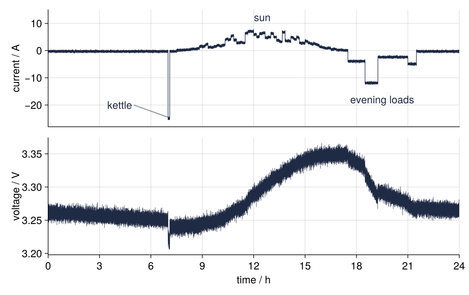
The current is the first witness. Add up amperes times seconds and you get a smooth charge, the method called coulomb counting. This sensor, though, reads 0.10 A high, and a bias does not average out: over the day it piles up 2.40 Ah that never reached the cell, and at midnight the count stands 4.78 % of the capacity above the truth, although it started from the truth.

The voltage is the second. The open-circuit voltage, the voltage of the cell at rest, climbs with the charge, so a curve converts one into the other. For this chemistry the curve is nearly level, 2 mV per percent, and the voltmeter's 5 mV of noise amount to 2.5 % of charge per reading. Under load the reading also holds the drop across the internal resistance \(R_0\): the kettle moves the reading 25.0 mV, and the curve mistakes that for 12.5 % of charge. Read at face value, the voltage misses by 3.12 % RMS and jumps by up to 19.9 %. Subtracting the resistance drop removes the jumps but not the noise: 2.51 % RMS.

Each witness is good where the other is bad. Counting barely changes its error from one second to the next and drifts over hours; the voltage never drifts and is off on every single reading. How should the two be combined, and with what weight at each moment? The Kalman filter's answer is a weighting by variances, recomputed at every reading, so the weights shift through the day.

The idea: multiply what you expect by what you measure

The filter keeps a state, the list of quantities it estimates. For now the state is one number, the charge; a second entry joins it later. Every second begins with a prediction: take the last estimate and add the charge that the counted current moved since. The prediction's mean is therefore coulomb counting, but the filter carries more than a mean. It carries a bell curve, the best guess together with a width that says how far off the guess may be.

To turn current into charge the filter uses \(c = 1\ \text{s}/(3600 \cdot 50\ \text{Ah}) \approx 5.6 \times 10^{-6}\) per ampere, the fraction of the 50 Ah that one ampere moves in one second. The counted current carries 0.2 A of noise, so each second blurs the charge by \(0.2c\), and the variance that every prediction step adds to the bell is \(q = (0.2\ \text{A} \cdot c)^2 = 1.2 \times 10^{-12}\). Both are fractions of the capacity, not percent: \(\sqrt q\) is \(1.1 \times 10^{-4}\) % of charge per second. And \(q\) holds only what the filter has been told, the noise. The 0.1 A offset is not in it, because the filter does not know there is one.

The measurement is a second bell: the voltage with the resistance drop removed, converted to charge through the curve, centered on the reading, with a width of 2.5 %. Multiply the two bells and you have the new estimate.

That multiplication is Bayes' rule. The prediction says how plausible each charge was before the reading arrived, the prior; the voltage says how likely this particular reading would be at each charge, the likelihood; and after the reading each charge is as plausible as prior times likelihood, renormalized. The likelihood may ignore the counting because the two sensors err independently: the voltage noise does not care how wrong the counting was. So the bells multiply as they stand, and the result is again a bell, narrower than either. Inverse variances add, \(1/\sigma^2 = 1/\sigma_-^2 + 1/\sigma_z^2\), where \(\sigma_-\) belongs to the prediction and \(\sigma_z\) to the measurement. The new mean averages the two old ones with the weights \(1/\sigma_-^2\) and \(1/\sigma_z^2\), so the narrower bell pulls harder. Were all \(n\) readings equally wide, this would reduce to an ordinary average whose width shrinks as \(\sigma/\sqrt n\), as the Python tutorial on the standard error shows.

The fraction of the gap between prediction and measurement that the estimate moves is the gain, \(K = \sigma_-^2/(\sigma_-^2 + \sigma_z^2)\). At \(K = 1\) the filter believes the voltage outright; at \(K = 0\) it keeps the count.

At midnight the system wakes up with a guess of 50 ± 10 % and no better. The figure draws prediction, voltage, and product at readings 1, 2, and 100, every curve scaled to the same peak height so that only the widths differ:

Show code

Copy

predict(x, P, u, q) = (x + c * u, P + q)

function update(x, P, z, r)
    K = P / (P + r)
    return x + K * (z - x), (1 - K) * P, K
end

q = (SIGMA_I * c)^2                                # what the counted current's noise adds per second
r = (SIGMA_V / K_OCV)^2                            # one voltage reading, in charge units

function first_readings(n)
    x, P = 0.5, 0.1^2                              # the wake-up guess: 50 ± 10 %
    keep = Dict{Int, NamedTuple}()
    for k in 1:n
        x_pred, P_pred = predict(x, P, I_m[k], q)
        x, P, K = update(x_pred, P_pred, soc_volt_r[k], r)
        keep[k] = (; x_pred, P_pred, z = soc_volt_r[k], x, P, K)
    end
    return keep
end
keep = first_readings(1000)

println("reading   prediction width   voltage width     gain   product width")
for n in [1, 2, 100, 1000]
    s = keep[n]
    @printf("%7d   %14.2f %%   %11.2f %%   %6.3f   %11.2f %%\n",
            n, 100 * sqrt(s.P_pred), 100 * sqrt(r), s.K, 100 * sqrt(s.P))
end
@printf("widening of the prediction per second at reading 100: %.1e of its width\n", q / (2 * keep[100].P))
@printf("c = %.1e per ampere, q = %.1e per second, sqrt(q) = %.1e %% of charge\n", c, q, 100 * sqrt(q))

soc_grid = range(20, 60, length = 4000)
bell(mean, var) = exp.(-0.5 .* (soc_grid .- 100 * mean) .^ 2 ./ (1e4 * var))
floor0 = zeros(length(soc_grid))

fig = Figure(size = (770, 726))
panels = [Axis(fig[i, 1], yticks = [0, 0.5, 1]) for i in 1:3]
for (ax, n) in zip(panels, [1, 2, 100])
    s = keep[n]
    vlines!(ax, [100 * soc[n]], ymax = 1.1 / 1.55, color = MUTED, linewidth = 1.5, linestyle = :dash)  # stops below the text
    lines!(ax, soc_grid, bell(s.x_pred, s.P_pred), color = SECOND)
    band!(ax, soc_grid, floor0, bell(s.z, r), color = (MUTED, 0.3))
    band!(ax, soc_grid, floor0, bell(s.x, s.P), color = (ACCENT, 0.35))
    lines!(ax, soc_grid, bell(s.x, s.P), color = ACCENT)
    text!(ax, 0.01, 0.96, text = @sprintf("reading %d, gain %.3f", n, s.K), space = :relative, align = (:left, :top))
    text!(ax, 0.99, 0.96, space = :relative, align = (:right, :top),
          text = @sprintf("widths: prediction %.2f %%, voltage %.2f %%\nproduct %.2f %%",
                          100 * sqrt(s.P_pred), 100 * sqrt(r), 100 * sqrt(s.P)))
    ylims!(ax, 0, 1.55)
end
x100 = 100 * keep[100].x
lines!(panels[3], [37.6, x100 + 0.3], [0.55, 0.75], color = MUTED, linewidth = 1.5)
text!(panels[3], 38, 0.55, text = "prediction and product\non top of each other", align = (:left, :center), color = INK)
Legend(fig[0, 1],
       [LineElement(color = SECOND), PolyElement(color = (MUTED, 0.3)),
        [PolyElement(color = (ACCENT, 0.35)), LineElement(color = ACCENT)],
        LineElement(color = MUTED, linestyle = :dash)],
       ["prediction", "voltage", "product", "true charge"],
       orientation = :horizontal, framevisible = false, halign = :left, tellwidth = false)
linkxaxes!(panels...)
hidexdecorations!.(panels[1:2], grid = false)
xlims!(panels[3], 20, 60)
panels[2].ylabel = "relative density"
panels[3].xlabel = "state of charge / %"
fig

reading   prediction width   voltage width     gain   product width
      1            10.00 %          2.50 %    0.941          2.43 %
      2             2.43 %          2.50 %    0.485          1.74 %
    100             0.25 %          2.50 %    0.010          0.25 %
   1000             0.08 %          2.50 %    0.001          0.08 %
widening of the prediction per second at reading 100: 9.9e-08 of its width
c = 5.6e-06 per ampere, q = 1.2e-12 per second, sqrt(q) = 1.1e-04 % of charge

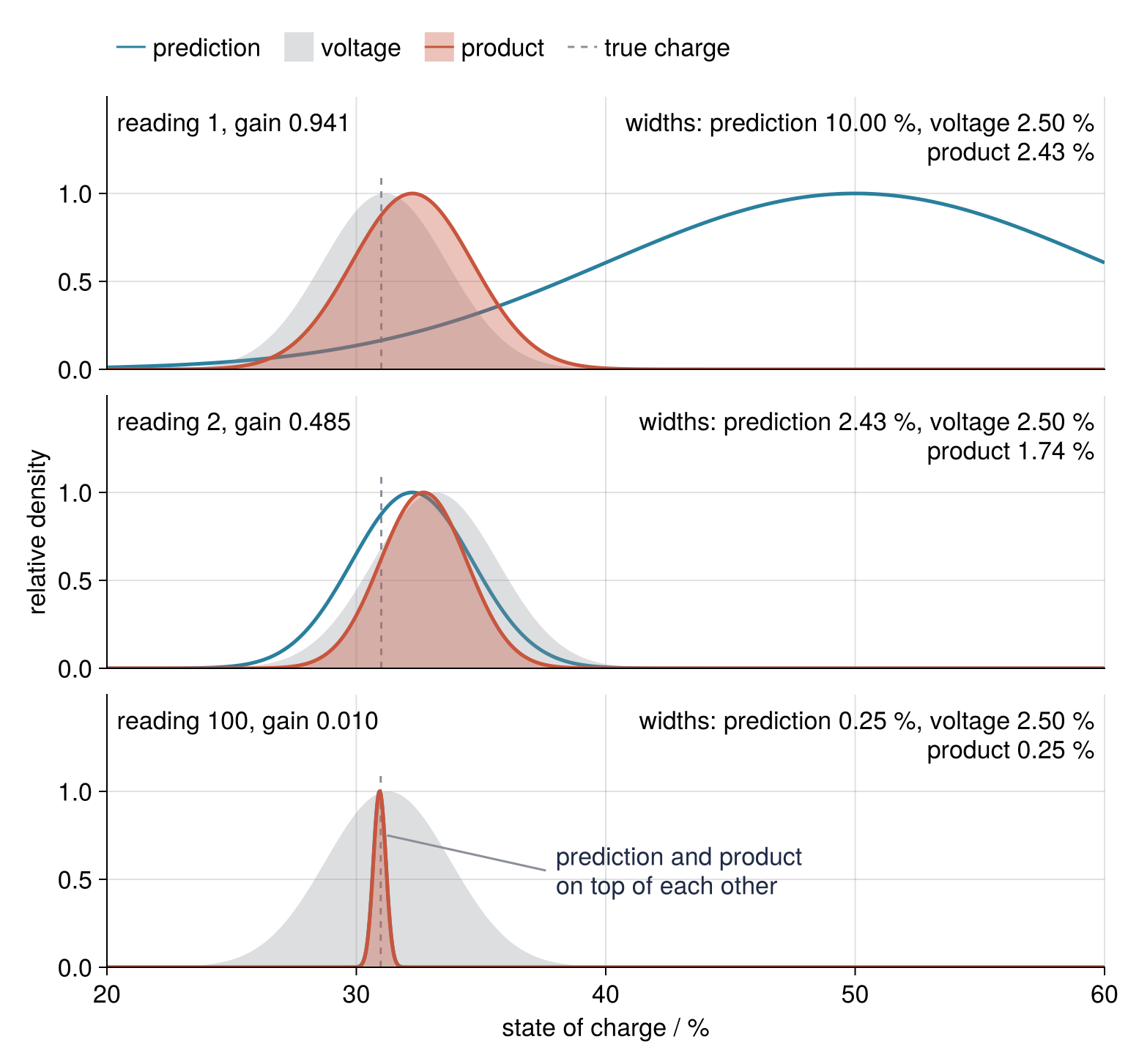
On reading 1 the prediction spans 10 % against the voltage's 2.50 %; with a gain of 0.941 the product lands almost on the measurement. One second later the prediction, reading 1's product widened by \(q\), has shrunk to 2.43 %, about the voltage's width, and with a gain of 0.485 the product falls halfway. By reading 100 the prediction has narrowed to 0.25 % and the gain to 0.010: the voltage now pulls the estimate one percent of the way toward itself. Nothing happened to the voltmeter. The prediction improved, because it now stands on every reading before it.

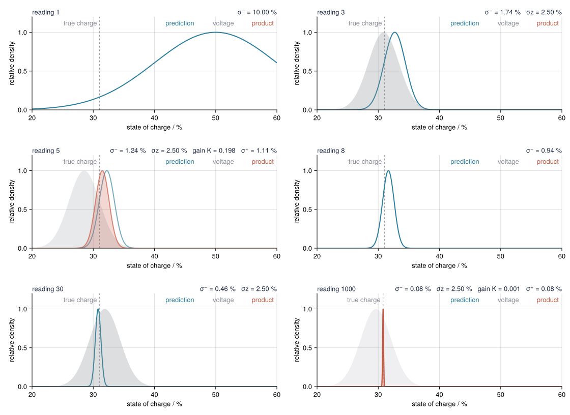
Each prediction step does widen the bell by \(q\), but at reading 100 the width grows by \(9.9 \times 10^{-8}\) of itself per second, which no plot can show; with \(q\) that small the gain falls almost like \(1/n\), a point the Formalization returns to. The animation writes the widths out as numbers instead:

# Kalman update: the battery filter waking up at midnight, one reading at a time.
# For readings 1 to 8, 10, 30, 100, and 1000 of the one-state filter, each reading is
# shown in three held states: the prediction alone, the voltage reading appearing, and
# the product forming while the other two fade. Every curve is scaled to a peak of 1.
# The data are those of the tutorial (same constants, seed, and order of draws, copied
# here rather than included). Run from this directory, in the repository's Julia project:
#
#     JULIA_PROJECT=../../../../.. julia scene.jl
#
# Writes ../../assets/kalman-update.gif.
using CairoMakie, Random, Printf

const INK, ACCENT, SECOND, MUTED = "#1f2a44", "#c8553d", "#2a7f9e", "#8a8f98"
const OUT = joinpath(@__DIR__, "..", "..", "assets", "kalman-update.gif")

# ---- data, as in the tutorial's setup cell
const CAPACITY_AH, DT = 50.0, 1.0
const V0, K_OCV, R0_OHM = 3.20, 0.20, 1.0e-3
const OFFSET_A, SIGMA_I, SIGMA_V = 0.10, 0.2, 5e-3
const SOC0, N = 0.31, 86_400
rng = Xoshiro(220)
t = (1:N) .* DT
hour = (t .- DT) ./ 3600
clouds = 0.35 .+ 0.65 .* rand(rng, 144)
I_true = fill(-0.4, N)
I_true[7.0 .<= hour .< 7.1] .= -25.0
sun = 7.5 .<= hour .< 17.5
I_true[sun] .= 8.0 .* sin.(π .* (hour[sun] .- 7.5) ./ 10) .^ 2 .* clouds[floor.(Int, 6 .* hour[sun]) .+ 1]
for (start, stop, amps) in [(17.5, 18.5, -4.0), (18.5, 19.25, -12.0), (19.25, 21.0, -2.5), (21.0, 21.5, -5.0)]
    I_true[start .<= hour .< stop] .= amps
end
c = DT / (3600 * CAPACITY_AH)
soc = SOC0 .+ c .* cumsum(I_true)
I_m = I_true .+ OFFSET_A .+ SIGMA_I .* randn(rng, N)
V = V0 .+ K_OCV .* soc .+ R0_OHM .* I_true .+ SIGMA_V .* randn(rng, N)
z = (V .- V0 .- R0_OHM .* I_m) ./ K_OCV

# ---- the one-state filter for the first 1000 readings, keeping every intermediate
q, r = (SIGMA_I * c)^2, (SIGMA_V / K_OCV)^2
steps = let x = 0.5, P = 0.1^2
    map(1:1000) do k
        x_pred, P_pred = x + c * I_m[k], P + q
        K = P_pred / (P_pred + r)
        x, P = x_pred + K * (z[k] - x_pred), (1 - K) * P_pred
        (; n = k, x_pred, s_pred = sqrt(P_pred), z = z[k], s_z = sqrt(r), K, x, s = sqrt(P), truth = soc[k])
    end
end

shown = [1, 2, 3, 4, 5, 6, 7, 8, 10, 30, 100, 1000]
frames = [(n, phase) for n in shown for phase in 0:8]   # three frames per held state

x_grid = range(20, 60, length = 4000)                    # fine enough for a 0.08 % bell
bell(mean, sd) = exp.(-0.5 .* ((x_grid .- 100 * mean) ./ (100 * sd)) .^ 2)
floor0 = zeros(length(x_grid))

set_theme!(Theme(
    fontsize = 13,
    Axis = (topspinevisible = false, rightspinevisible = false, xgridvisible = true, ygridvisible = true),
))
fig = Figure(size = (560, 272))
ax = Axis(fig[2, 1], xlabel = "state of charge / %", ylabel = "relative density", yticks = [0, 0.5, 1])
limits!(ax, 20, 60, 0, 1.2)

# Everything that changes between frames is an Observable, set from (reading, phase)
frame = Observable(frames[1])
s = @lift steps[$frame[1]]
phase = @lift $frame[2]
fade = @lift $phase < 6 ? 1.0 : 1.0 - 0.18 * ($phase - 5)   # 0.82, 0.64, 0.46 while the product forms
grow = @lift $phase < 6 ? 0.0 : ($phase - 5) / 3

vlines!(ax, @lift([100 * $s.truth]), color = MUTED, linewidth = 1.2, linestyle = :dash)
lines!(ax, x_grid, @lift(bell($s.x_pred, $s.s_pred)), color = @lift((SECOND, $fade)), linewidth = 2)
band!(ax, x_grid, floor0, @lift(bell($s.z, $s.s_z)), color = @lift((MUTED, 0.3 * $fade)),
      visible = @lift($phase >= 3))
band!(ax, x_grid, floor0, @lift(bell($s.x, $s.s)), color = @lift((ACCENT, 0.35 * $grow)))
lines!(ax, x_grid, @lift(bell($s.x, $s.s)), color = @lift((ACCENT, $grow)), linewidth = 2)

# The key words in their colors, and the numbers of the current reading above the axis
text!(ax, @lift(100 * $s.truth - 0.4), 1.12, text = "true charge", color = MUTED, align = (:right, :center))
for (x_key, word, color) in [(46.5, "prediction", SECOND), (53, "voltage", MUTED), (59.5, "product", ACCENT)]
    text!(ax, x_key, 1.12, text = word, color = color, align = (:right, :center))
end
Label(fig[1, 1], @lift(@sprintf("reading %d", $s.n)), halign = :left, tellwidth = false, color = INK)
numbers = @lift begin
    line = @sprintf("σ⁻ = %.2f %%", 100 * $s.s_pred)
    $phase >= 3 && (line *= @sprintf("   σz = %.2f %%", 100 * $s.s_z))
    $phase >= 6 && (line *= @sprintf("   gain K = %.3f   σ⁺ = %.2f %%", $s.K, 100 * $s.s))
    line
end
Label(fig[1, 1], numbers, halign = :right, tellwidth = false, color = INK)
rowgap!(fig.layout, 1, 2)                               # the numbers sit close above the axis

record(fig, OUT, frames; framerate = 12, px_per_unit = 1) do f
    frame[] = f
end
@printf("wrote %s: %d frames, %d kB\n", OUT, length(frames), filesize(OUT) ÷ 1024)

By reading 1000 the gain is down to 0.001, and the filter hardly listens to the voltage anymore. That is correct only if counting really is as precise as its width claims, and a sensor 0.1 A off makes the claim false.

Formalization

Write \(\hat x\) for the state estimate from the idea, \(u\) for the counted current, and \(z\) for the measurement in charge units. One second of the filter is then

\(P\) is the bell's squared width, the variance of the error in \(\hat x\); hence \(P^- = \sigma_-^2\) and \(r = \sigma_z^2\).

For several tracked quantities, \(x\) becomes a vector, one entry per quantity, and the steps read

\(F\) carries the state one step forward, \(B\) brings in the input, and \(H\) gives the reading the meter should show for a given state. With a single entry, \(F = 1\), \(B = c\), and \(H = 1\) give back the scalar equations. The battery's own \(F\), \(B\), \(H\) follow in the third consequence.

\(P\) is now the covariance matrix of the errors. Its diagonal holds the variance of each entry; an off-diagonal element tells whether two entries err in the same direction (positive), in opposite ones (negative), or independently (zero). \(FPF^\top\) moves the old errors forward as \(F\) moves the state, and \(Q\) adds fresh ones. That is propagation of uncertainty by the linear rule (in Python) in matrix form, with \(F\) as the Jacobian.

The gain is a ratio of variances, and without process noise the filter is an average. Process noise is \(q\), the fresh error each prediction adds. Without it every reading weighs the same, and a plain mean of \(n\) readings gives its newest one the weight \(1/n\), so the gain at reading \(n\) is close to \(1/n\): 0.010 at reading 100, 0.001 at reading 1000.

A filter is only as honest as its \(q\). Run the one-state filter through the whole day, with \(q = 1.2 \times 10^{-12}\):

Show code

Copy

function scalar_filter(q)
    x, P = 0.5, 0.1^2
    xs, Ps, Ks = zeros(N), zeros(N), zeros(N)
    for k in 1:N
        x, P = predict(x, P, I_m[k], q)
        x, P, Ks[k] = update(x, P, soc_volt_r[k], r)
        xs[k], Ps[k] = x, P
    end
    return xs, Ps, Ks
end

soc_1, P_1, K_1 = scalar_filter(q)
err_1 = 100 .* (soc_1 .- soc)
@printf("q                        %.1e per second\n", q)
@printf("gain at midnight         %.1e, so a memory of 1/K = %.0f readings, %.1f h\n",
        K_1[end], 1 / K_1[end], DT / K_1[end] / 3600)
@printf("reported width           %.3f %%\n", 100 * sqrt(P_1[end]))
@printf("error at midnight        %+.2f %%\n", err_1[end])
@printf("RMS error over the day   %.2f %%\n", rms(soc_1 .- soc))
soc_9, _, _ = scalar_filter(1e-9)
@printf("same with q = 1e-9       RMS %.2f %%\n", rms(soc_9 .- soc))

fig = Figure(size = (770, 374))
ax = Axis(fig[1, 1], xlabel = "time / h", ylabel = "error / %", xticks = 0:3:24, yticks = -2:2:6)
hlines!(ax, [0], color = MUTED, linewidth = 1.5)
err_count = 100 .* (soc_count .- soc)
lines!(ax, hours, err_count, color = SECOND)
text!(ax, 23.8, err_count[end] + 0.3, text = "counting", align = (:right, :bottom), color = SECOND)
band_1 = 200 .* sqrt.(P_1)                         # ±2σ, in percent
band!(ax, hours, err_1 .- band_1, err_1 .+ band_1, color = (ACCENT, 0.15))
lines!(ax, hours, err_1, color = ACCENT)
text!(ax, 23.8, err_1[end] + 0.35, align = (:right, :bottom), color = ACCENT,
      text = @sprintf("one-state filter\nreported width %.3f %%\noff by %.2f %%", 100 * sqrt(P_1[end]), err_1[end]))
limits!(ax, 0, 24, -3, 6)
fig

q                        1.2e-12 per second
gain at midnight         4.4e-05, so a memory of 1/K = 22480 readings, 6.2 h
reported width           0.017 %
error at midnight        +1.14 %
RMS error over the day   0.82 %
same with q = 1e-9       RMS 0.07 %

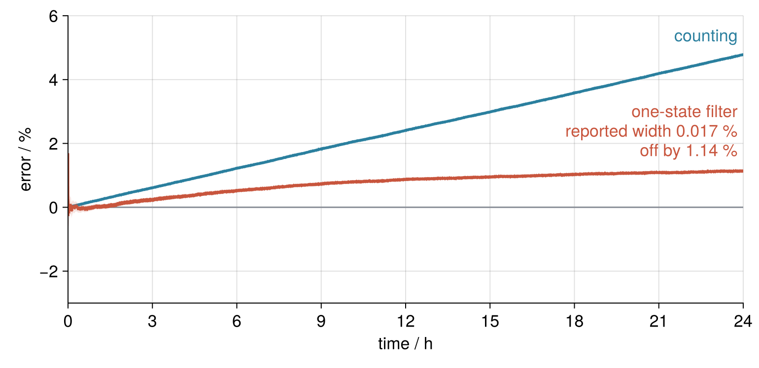
That \(q\) was built from the 0.2 A of noise and knows nothing of the 0.1 A offset. By midnight the gain has dropped to \(4.4 \times 10^{-5}\), and read backward, a gain \(K\) acts like a mean over the last \(1/K\) readings: here 22,480 of them, or 6.2 h. Its claimed width is 0.017 %, yet it ends 1.14 % off, with 0.82 % RMS over the day: sure and wrong. Raising \(q\) by hand to \(10^{-9}\) cuts the RMS to 0.07 %; the filter then learns that something drifts, never what.

Put the offset into the state and the drift disappears. Give the offset \(b\) its own entry, \(x = (\text{SOC}, b)\), measure in volts with the counted resistance drop removed, \(z = V - V_0 - R_0 I_m\), and the battery reads

where \(k = 0.20\) V per unit charge is the curve's slope. Since \(I_m\) equals the true current plus \(b\), a step of counting adds \(c\,I_m\) and has to take \(c\,b\) back out: the \(-c\) in \(F\). The second row and the zero in \(Q\) keep \(b\) constant. What the voltmeter reads is \(k\,\text{SOC} + R_0 I\); subtracting \(R_0 I_m = R_0 (I + b)\) leaves \(-R_0 b\), the \(-R_0\) in \(H\). Starting values: charge 50 ± 10 %, offset 0 ± 0.2 A.

Show code

Copy

function kalman(x, P, F, B, H, Q, R, u, z)
    # The five equations, once per reading; returns the estimates and their covariances.
    n = length(x)
    xs, Ps = zeros(length(z), n), zeros(length(z), n, n)
    for k in eachindex(z)
        x, P = F * x + B * u[k], F * P * F' + Q             # predict
        S = H * P * H' + R
        K = (P * H') / S                                    # P H' S⁻¹ by right division, no inverse
        x, P = x + K * ([z[k]] - H * x), (I - K * H) * P    # update; z[k] as a one-element vector
        xs[k, :], Ps[k, :, :] = x, P
    end
    return xs, Ps
end

F = [1.0 -c; 0.0 1.0]
B = [c, 0.0]
H = [K_OCV -R0_OHM]                                # a 1 × 2 matrix
Q = diagm([(SIGMA_I * c)^2, 0.0])
R = fill(SIGMA_V^2, 1, 1)
z = V .- V0 .- R0_OHM .* I_m
xs, Ps = kalman([0.5, 0.0], diagm([0.1^2, 0.2^2]), F, B, H, Q, R, I_m, z)

b_hat, b_sd = xs[:, 2], sqrt.(Ps[:, 2, 2])
corr = Ps[:, 1, 2] ./ sqrt.(Ps[:, 1, 1] .* Ps[:, 2, 2])
println("after    offset estimate      correlation of charge and offset errors")
for h in [1, 4, 24]
    k = round(Int, h * 3600 / DT)
    @printf("%3d h    %.3f ± %.3f A    %+.2f\n", h, b_hat[k], b_sd[k], corr[k])
end
@printf("the true offset in one reading: %.1f mV, against %.0f mV of noise\n", 1e3 * R0_OHM * OFFSET_A, 1e3 * SIGMA_V)
drift = OFFSET_A * 3600 * c                        # what the offset adds to an uncorrected count in 1 h
@printf("its drift of the count in 1 h: %.2f %% of charge, %.2f mV on the voltage, against %.2f mV of noise in an hour's mean\n",
        100 * drift, 1e3 * K_OCV * drift, 1e3 * SIGMA_V / sqrt(3600 / DT))

fig = Figure(size = (770, 374))
ax = Axis(fig[1, 1], xlabel = "time / h", ylabel = "offset / A", xticks = 0:3:24)
hlines!(ax, [OFFSET_A], color = MUTED, linewidth = 1.5, linestyle = :dash)
band!(ax, hours, b_hat .- 2 .* b_sd, b_hat .+ 2 .* b_sd, color = (ACCENT, 0.15))
lines!(ax, hours, b_hat, color = ACCENT)
text!(ax, 23.8, OFFSET_A + 0.02, text = "true offset 0.1 A", align = (:right, :bottom), color = MUTED)
limits!(ax, 0, 24, -0.3, 0.5)
fig

after    offset estimate      correlation of charge and offset errors
  1 h    0.082 ± 0.068 A    -0.63
  4 h    0.097 ± 0.009 A    -0.81
 24 h    0.099 ± 0.001 A    -0.55
the true offset in one reading: 0.1 mV, against 5 mV of noise
its drift of the count in 1 h: 0.20 % of charge, 0.40 mV on the voltage, against 0.08 mV of noise in an hour's mean

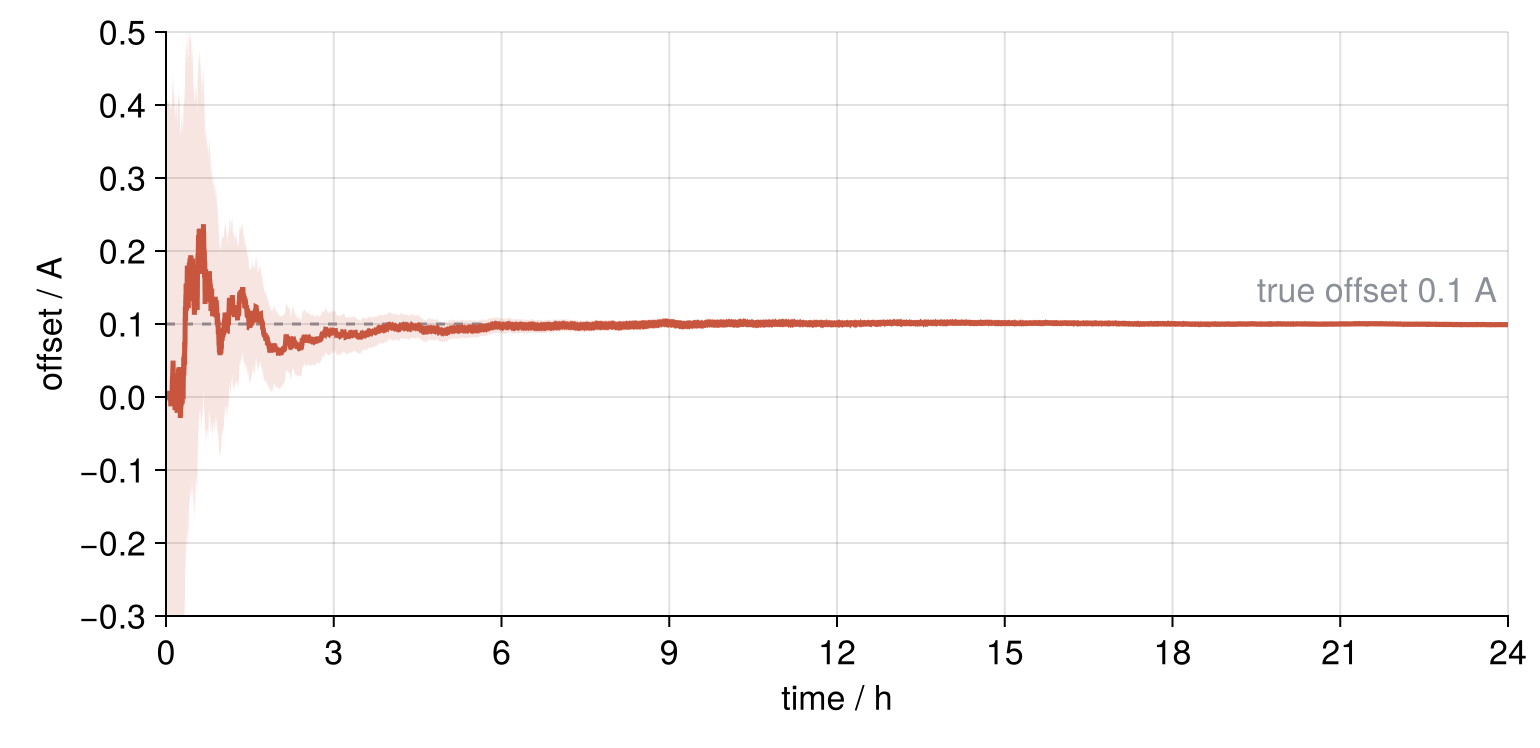
After 1 h the filter puts the offset at 0.082 ± 0.068 A, after 4 h at 0.097 ± 0.009 A, and by midnight at 0.099 ± 0.001 A. In a single reading the offset is \(-R_0 b\), 0.1 mV under 5 mV of noise. The count gives it away. With the offset guessed too low, the count runs high, and the voltage keeps landing below the prediction, hour after hour: in 1 h the 0.1 A moves the count by 0.20 % of charge, 0.40 mV on the voltage, against 0.08 mV of noise in an hour's mean.

The off-diagonal element of \(P\) turns that shortfall into an offset. Every second \(FPF^\top\) adds \(-c\) times the offset's variance to it. Divided by both widths it is the correlation, −0.63 at 1 h and −0.81 at 4 h. Through \(P^-H^\top\), the offset's entry of \(K\) has the sign of \(k\) times that element minus \(R_0\) times the offset's variance, negative once the element is: a reading below the prediction lowers the charge and raises the offset. By midnight the offset is settled, the charge error is mostly fresh current noise, and the correlation is back to −0.55.

See it in code

No package does this for you, and none is needed: the filter is the five equations, the function kalman of about 15 lines in the hidden cell above, with LinearAlgebra's right division / for the gain and its I for the identity. That one function ran the day; its estimate and the two witnesses, set against the truth:

Show code

Copy

soc_kf = xs[:, 1]
println("estimate          RMS error   error at midnight")
for (name, est) in [("counting", soc_count), ("voltage alone", soc_volt), ("Kalman filter", soc_kf)]
    @printf("%-15s   %7.2f %%   %+15.2f %%\n", name, rms(est .- soc), 100 * (est[end] - soc[end]))
end
late = abs.(soc_kf .- soc)[61:end]                 # after the first minute
worst = argmax(late)
@printf("largest filter error after the first minute: %.2f %% (at %.0f s)\n", 100 * late[worst], t[60 + worst])
@printf("the filter is %.0f times closer than the better witness (RMS)\n",
        min(rms(soc_count .- soc), rms(soc_volt .- soc)) / rms(soc_kf .- soc))

fig = Figure(size = (770, 506))
ax1 = Axis(fig[1, 1], ylabel = "charge / %", yticks = 20:20:80)
ax2 = Axis(fig[2, 1], xlabel = "time / h", ylabel = "error / %", xticks = 0:3:24)
linkxaxes!(ax1, ax2)
hidexdecorations!(ax1, grid = false)
lines!(ax1, hours, 100 .* soc_volt, color = (MUTED, 0.45), linewidth = 0.5)
lines!(ax1, hours, 100 .* soc, color = INK, linewidth = 4.9)
lines!(ax1, hours, 100 .* soc_count, color = SECOND)
lines!(ax1, hours, 100 .* soc_kf, color = ACCENT, linewidth = 2.1)
ylims!(ax1, 10, 90)
Legend(fig[0, 1],
       [LineElement(color = INK, linewidth = 4.9), LineElement(color = SECOND), LineElement(color = ACCENT),
        LineElement(color = MUTED, linewidth = 2.5)],          # the voltage key at full alpha, not a hairline
       ["truth", "counting", "Kalman filter", "voltage alone"],
       orientation = :horizontal, framevisible = false, halign = :left, tellwidth = false)
lines!(ax2, hours, 100 .* (soc_volt .- soc), color = (MUTED, 0.45), linewidth = 0.5)
lines!(ax2, hours, 100 .* (soc_count .- soc), color = SECOND)
lines!(ax2, hours, 100 .* (soc_kf .- soc), color = ACCENT)
for (x_text, al, name, est, color) in [(0.2, :left, "RMS: voltage alone", soc_volt, MUTED),
                                       (12.6, :center, "counting", soc_count, SECOND),
                                       (23.8, :right, "Kalman filter", soc_kf, ACCENT)]
    text!(ax2, x_text, 14.5, text = @sprintf("%s %.2f %%", name, rms(est .- soc)), align = (al, :center), color = color)
end
limits!(ax2, 0, 24, -16, 17)
ax1.yticklabelspace = ax2.yticklabelspace = maximum(tight_yticklabel_spacing!, (ax1, ax2))  # align the y labels
fig

estimate          RMS error   error at midnight
counting             2.77 %             +4.78 %
voltage alone        3.12 %             -2.04 %
Kalman filter        0.04 %             +0.00 %
largest filter error after the first minute: 0.19 % (at 125 s)
the filter is 72 times closer than the better witness (RMS)

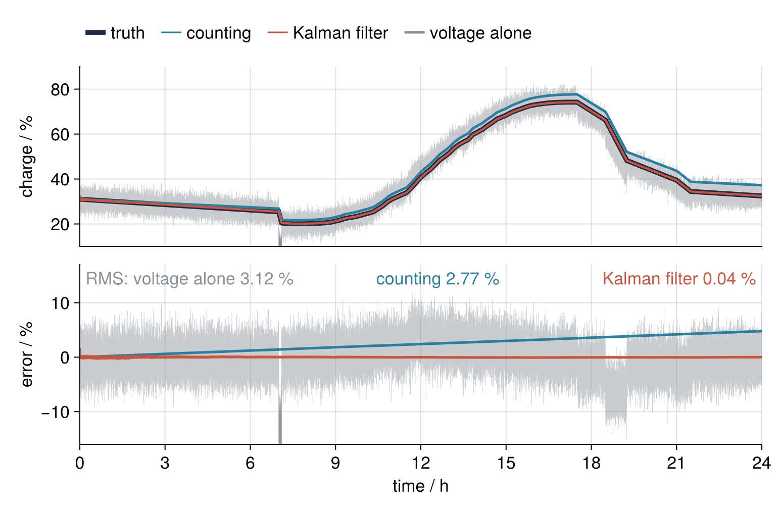
Counting misses by 2.77 % RMS, the voltage alone by 3.12 %, and the filter by 0.04 %, 72 times closer than the better witness. After its first minute the filter is never more than 0.19 % off, and that worst moment, at 125 s, comes while the offset is still unknown. Do not expect this from a real cell. Here the model behind the filter is exactly right: the curve is straight, and the filter knows \(R_0\) and the capacity because the data were generated from them. On a real cell the open-circuit curve bends and shifts with temperature, so battery management in practice uses the extended Kalman filter, which linearizes the curve afresh at every step.

Where it shows up

Wherever a model predicts how some state evolves and a sensor sees part of that state through noise, the battery's problem returns under another name.

• Battery management. The extended Kalman filter in an electric vehicle estimates, besides the charge, the voltages across the resistor-capacitor pairs of the cell's equivalent circuit. The standard reference for these filters is the work of Gregory Plett.
• Navigation. Stanley Schmidt at NASA Ames extended the filter to nonlinear orbits, and the Apollo guidance computer used it on the way to the Moon. The navigation unit of a car or a drone blends satellite fixes, noisy but free of drift, with inertial sensors, smooth but drifting: the same pair of witnesses as in the battery.
• Particle physics. Detectors at CERN reconstruct the path of a charged particle with a Kalman filter, whose state holds position, direction, and the track's curvature in the magnetic field, from which the momentum follows. Each detector layer is a measurement, the step to the next layer is the prediction, and multiple scattering in the material is the process noise.
• Weather and climate. Forecast centers fold millions of observations into a running weather model, which is called data assimilation. Its ensemble variant of the filter stands a set of model runs in for \(P\), since a state of hundreds of millions of entries would make \(P\) that number squared.
• Neuroscience. Brain-computer interfaces take the velocity of a hand or a cursor as the state and the firing rates of neurons in motor cortex as the measurement. The filter predicts the intended movement and corrects it with what the neurons report.
• Chemical engineering. A reactor's concentrations are tracked from a temperature measured every second and an analyzer that returns a concentration every few minutes. Between analyses the model carries the estimate forward, and each analysis pulls it back.

What carries over to each of them is what the battery showed: at every step, weigh the prediction against the measurement by their variances, and give any constant unknown, an offset or a drift, its own entry in the state so that the filter can learn it.

Further reading

• LinearAlgebra in the Julia standard library documentation, for right division /, backslash \, and the identity I; with them the gain needs no explicit inverse.
• Where the filter first appeared: R. E. Kalman, "A New Approach to Linear Filtering and Prediction Problems" (1960), Journal of Basic Engineering 82, pages 35 to 45.
• Roger Labbe's free online book Kalman and Bayesian Filters in Python builds the filter out of bell curves step by step and reads well from Julia. For the extended filter on real cells: Gregory L. Plett, Battery Management Systems, Volume II: Equivalent-Circuit Methods, Artech House, 2015.
• On this site: The Kalman filter: a battery's charge from a drifting current and noisy voltage, the same tutorial in Python; ModelingToolkit.jl from the ground up: a DC motor under speed control, the other control tutorial in Julia; Eigenvalues with LinearAlgebra: normal modes of coupled oscillators, for the package; The standard error of the mean: why four times the data halves the error, in Python; Uncertainty propagation by sampling with NumPy: beyond the linear rule, in Python.
• Download the notebook. It was executed with the library versions in the header.