Uncertainty propagation by sampling with NumPy: beyond the linear rule

The problem: how uncertain is g, and how uncertain is a heat capacity?

A pendulum of length L = 1.000 ± 0.002 m swings with a period T = 2.006 ± 0.005 s, so g = 4π²L/T² = 9.811 m/s². The lab report also wants the uncertainty of g. Getting it from the uncertainties of the inputs is called uncertainty propagation, and the lab manual's answer is a formula with partial derivatives that assumes g depends nearly linearly on L and T over their scatter. There is a route that needs neither assumption nor derivatives: draw a hundred thousand plausible values of L and T, compute g for each, and look at the spread. For the pendulum both routes give ± 0.053 m/s².

The second example is where they part. A small calorimeter takes up Q = 50.0 ± 0.5 J and warms by ΔT = 0.40 ± 0.10 K, the difference of two thermometer readings, so its heat capacity is C = Q/ΔT = 125 J/K. ΔT is only four of its own standard deviations above zero. The linear rule says ± 31 J/K; the samples say that the central 95 % of the possible values run from 84 to 242 J/K, a long tail to the right that no symmetric ± can describe.

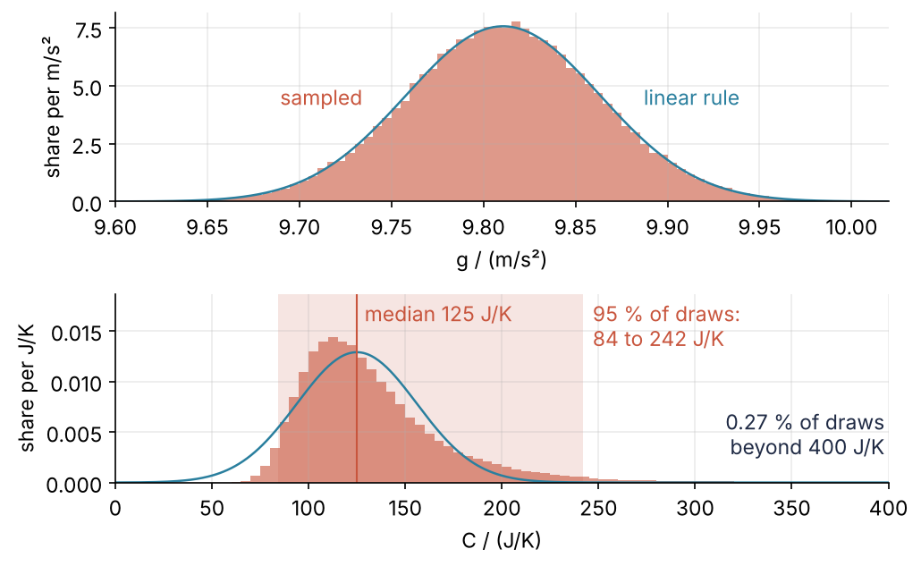
Histograms of 100,000 sampled results under the linear rule's normal curve. Top: g in m/s², the two coincide. Bottom: heat capacity C in J/K, the samples peak near 110 J/K with a long tail to the right, the curve reaches below every positive draw, and a line marks the median, 125 J/K, inside the 95 % interval of 84 to 242 J/K.

This is where we end up. Each panel is 100,000 draws of the inputs pushed through the formula, shown as a histogram, with the linear rule's answer drawn as a normal curve over it. Step 6 draws it from the arrays the steps before it build.

Setup

One generator, seeded once, serves every draw below:

import numpy as np
import matplotlib.pyplot as plt

rng = np.random.default_rng(1)   # every draw comes from this generator, in a fixed order
N = 100_000                      # draws per input

plt.rcParams.update({
    "figure.figsize": (7, 3.6), "figure.dpi": 110,
    "axes.spines.top": False, "axes.spines.right": False,
    "axes.grid": True, "grid.alpha": 0.25,
    "font.size": 11, "lines.linewidth": 1.8,
})
INK, ACCENT, SECOND, MUTED = "#1f2a44", "#c8553d", "#2a7f9e", "#8a8f98"

print(f"N = {N:,} draws per input, generator {type(rng.bit_generator).__name__}, seed 1")

N = 100,000 draws per input, generator PCG64, seed 1

Step 1: Draw each input around its measured value

A measurement written L = 1.000 ± 0.002 m makes a claim about repeats: measure again and you would get values scattered around 1.000 m with a standard deviation of 0.002 m. Sampling takes that claim literally. Each input becomes an array of N normal draws centered on its measured value, with its standard uncertainty as the standard deviation, drawn as in Random numbers with numpy.random. The standard error of the mean drew measurements around a known truth; here the truth is unknown, and the measured value stands in for it.

L = rng.normal(1.000, 0.002, N)   # m
T = rng.normal(2.006, 0.005, N)   # s

for name, x, unit in [("L", L, "m"), ("T", T, "s")]:
    print(f"{name} = {x.mean():.4f} ± {x.std(ddof=1):.4f} {unit}")

L = 1.0000 ± 0.0020 m
T = 2.0060 ± 0.0050 s

The draws reproduce the inputs to the last quoted digit, 1.0000 ± 0.0020 m and 2.0060 ± 0.0050 s.

Step 2: Push every draw through the formula

Each pair of draws, one L and one T, is one imagined repeat of the experiment. NumPy applies the formula to whole arrays, so one line gives 100,000 values of g, and their standard deviation (sd) is the uncertainty of g. The second print checks that N is large enough:

g = 4 * np.pi**2 * L / T**2

print(f"g = {g.mean():.3f} ± {g.std(ddof=1):.3f} m/s²   median {np.median(g):.3f} m/s²")
print(f"standard error of the mean of the draws: {g.std(ddof=1) / np.sqrt(N):.4f} m/s²")

g = 9.811 ± 0.053 m/s²   median 9.810 m/s²
standard error of the mean of the draws: 0.0002 m/s²

The result is g = 9.811 ± 0.053 m/s². The median, the value with half the draws below it, is 9.810 m/s², within 0.001 m/s² of the mean. The mean of the draws has its own sampling error, sd/√N = 0.0002 m/s², far below the last digit quoted.

Every formula goes through these two steps, so wrap them in a function. Write the formula as an ordinary Python function, def g_of(L, T) (a lambda works too), whose parameter names are the names of the inputs, and put the inputs in a dictionary from name to (value, uncertainty). Inside, propagate builds a dictionary draws with one array per name and calls f(**draws). The ** unpacks a dictionary into keyword arguments, so f(**{"L": a, "T": b}) is the call f(L=a, T=b). That is the one rule for your own formula: one parameter per input, named as in the dictionary.

def propagate(f, inputs, rng, N):
    draws = {name: rng.normal(value, sigma, N) for name, (value, sigma) in inputs.items()}
    return f(**draws)

def g_of(L, T):
    return 4 * np.pi**2 * L / T**2

pendulum = {"L": (1.000, 0.002), "T": (2.006, 0.005)}
g = propagate(g_of, pendulum, rng, N)
print(f"g = {g.mean():.3f} ± {g.std(ddof=1):.3f} m/s²")

g = 9.811 ± 0.053 m/s²

Fresh draws, the same 9.811 ± 0.053 m/s².

Step 3: Check against the linear rule with a numerical gradient

The lab manual's rule rests on one assumption: near the measured values, f is nearly a plane. A small error δxᵢ in input i then moves f by (∂f/∂xᵢ) δxᵢ, and independent errors add in variance, the rule the standard error tutorial used for the mean. Hence

\[\sigma_f^2 = \sum_i \left(\frac{\partial f}{\partial x_i}\,\sigma_i\right)^2 ,\]

with σᵢ the standard uncertainty of input i and σ_f that of the result. Deriving every ∂f/∂xᵢ by hand is where people make mistakes, and it has to be redone for each new formula. The computer gets it from a central difference: the change between f(xᵢ + h) and f(xᵢ − h), divided by 2h. I take h as a thousandth of that input's own uncertainty, σᵢ/1000, which is small on the scale where the rule claims f is a plane, and never zero. A fraction of the measured value would be zero for an input measured as 0, and Step 4 has one. The code keeps the measured values in a dictionary x0 and builds each shifted input as {**x0, name: value + h}: inside braces, ** copies every entry of x0, and the key written after it replaces one.

def linear_rule(f, inputs):
    x0 = {name: value for name, (value, sigma) in inputs.items()}
    variance = 0.0
    for name, (value, sigma) in inputs.items():
        h = sigma / 1000                   # never zero, even for an input measured as 0
        up = {**x0, name: value + h}
        down = {**x0, name: value - h}
        slope = (f(**up) - f(**down)) / (2 * h)
        variance += (slope * sigma) ** 2
    return f(**x0), np.sqrt(variance)

g_lin, sigma_g = linear_rule(g_of, pendulum)
print(f"linear rule  g = {g_lin:.3f} ± {sigma_g:.3f} m/s²   ({100 * sigma_g / g_lin:.2f} %)")
print(f"sampled      g = {g.mean():.3f} ± {g.std(ddof=1):.3f} m/s²")

linear rule  g = 9.811 ± 0.053 m/s²   (0.54 %)
sampled      g = 9.811 ± 0.053 m/s²

The two agree to the last digit. The relative uncertainty, 0.54 %, is also what the lab manual's shortcut for a power law gives, relative errors added in quadrature: 0.2 % from L and 2 × 0.25 % from T², since T enters squared. That shortcut is this rule, worked out once for products and powers.

Step 4: Draw a shared error source once

The calorimeter's ΔT = T₂ − T₁ comes from two readings of one thermometer, T₁ = 22.10 °C and T₂ = 22.50 °C. I assume each reading scatters by 0.07 K on its own, the spread of repeated readings of a steady bath, and that both share one calibration offset of 0.3 K, because it is the same thermometer. The standard error tutorial gave the remedy for a shared error: draw it once per experiment and add it to every reading that shares it. Here the offset becomes an input of its own, c, measured as 0 with an uncertainty of 0.3 K. Next to it, the wrong version gives each reading an offset of its own:

def dT_of(T1, T2, c):
    return (T2 + c) - (T1 + c)             # one offset, shared by both readings

def dT_separate(T1, T2, c1, c2):
    return (T2 + c2) - (T1 + c1)           # wrong: the same thermometer gets two offsets

thermometer = {"T1": (22.10, 0.07), "T2": (22.50, 0.07), "c": (0.0, 0.3)}
separate = {"T1": (22.10, 0.07), "T2": (22.50, 0.07), "c1": (0.0, 0.3), "c2": (0.0, 0.3)}

for label, f, inputs in [("drawn once", dT_of, thermometer), ("per reading", dT_separate, separate)]:
    dT = propagate(f, inputs, rng, N)
    print(f"offset {label:11s}  ΔT = {dT.mean():.2f} ± {dT.std(ddof=1):.3f} K   "
          f"at or below zero: {100 * np.mean(dT <= 0):4.1f} %")

dT_lin, sigma_dT = linear_rule(dT_of, thermometer)
print(f"linear rule with c    ΔT = {dT_lin:.2f} ± {sigma_dT:.3f} K")

offset drawn once   ΔT = 0.40 ± 0.099 K   at or below zero:  0.0 %
offset per reading  ΔT = 0.40 ± 0.435 K   at or below zero: 17.9 %
linear rule with c    ΔT = 0.40 ± 0.099 K

Drawn once, the offset cancels in the difference, and ΔT = 0.40 ± 0.099 K, the two reading errors in quadrature, 0.07 × √2. Drawn per reading, the spread is 0.435 K, and 17.9 % of the draws are at or below zero, which would make C = Q/ΔT meaningless. The linear rule needs the same treatment, and with c as an input it also returns 0.099 K, because ∂ΔT/∂c = 0.

Step 5: Report a skewed result with the median and a 95 % interval

Now the heat capacity, Q = 50.0 ± 0.5 J divided by the ΔT of Step 4, by both methods. **thermometer merges Step 4's inputs into the new dictionary:

def C_of(Q, T1, T2, c):
    return Q / dT_of(T1, T2, c)

calorimeter = {"Q": (50.0, 0.5), **thermometer}
C = propagate(C_of, calorimeter, rng, N)
C_lin, sigma_C = linear_rule(C_of, calorimeter)
C_med = np.median(C)
C_lo, C_hi = np.percentile(C, [2.5, 97.5])

print(f"linear rule   C = {C_lin:.0f} ± {sigma_C:.0f} J/K")
print(f"sampled       mean {C.mean():.0f} J/K   sd {C.std(ddof=1):.0f} J/K")
print(f"              median {C_med:.0f} J/K   95 % interval {C_lo:.0f} to {C_hi:.0f} J/K")

for name, y in [("g", g), ("C", C)]:
    lo, med, hi = np.percentile(y, [2.5, 50, 97.5])
    print(f"{name}: upper end {(hi - med) / (med - lo):.2f} times as far from the median as the lower end")

linear rule   C = 125 ± 31 J/K
sampled       mean 136 J/K   sd 278 J/K
              median 125 J/K   95 % interval 84 to 242 J/K
g: upper end 1.02 times as far from the median as the lower end
C: upper end 2.86 times as far from the median as the lower end

The linear rule says 125 ± 31 J/K. The samples give a mean of 136 J/K and an sd of 278 J/K, nine times the linear value, and neither can be trusted: over seeds 1 to 5 the sd runs from 53 to 5,133 J/K. The cause is the draws of ΔT near zero. A ΔT of 0.05 K gives C = 1,000 J/K, and a handful of such draws drags the mean and blows up the sd, which squares their distance.

The median, and the 2.5th and 97.5th percentiles that cut off the lowest and highest 2.5 % of the draws, do not care how far the extreme draws lie, only on which side. The median is 125 J/K and the interval 84 to 242 J/K, and over the same five seeds the median moves by 0.3 J/K and the interval's ends by less than 4 J/K. A normal distribution holds 95 % of its values within about two standard deviations, so the linear rule's interval is 125 ± 2 × 31 J/K, 63 to 187 J/K, too low at both ends.

When the mean and the median agree and the two ends of the interval lie at the same distance from the median to within about 10 %, report mean ± sd. A finer test is pointless: an uncertainty from a few dozen repeats is itself uncertain by more than 10 %. Otherwise report the median and the 95 % interval. The printed ratio is 1.02 for g and 2.86 for C, so C = 125 J/K, 95 % interval 84 to 242 J/K.

Step 6: Plot the sampled distributions against the linear rule

The bars are counts divided by N times the bin width, so they compare directly with the normal curve of the linear rule. density=True, as in the standard error tutorial, would rescale whatever lies inside the plotted range to area 1, and for C that range stops at 400 J/K:

def normal_curve(x, mu, sigma):
    return np.exp(-0.5 * ((x - mu) / sigma) ** 2) / (sigma * np.sqrt(2 * np.pi))

fig, (ax_g, ax_C) = plt.subplots(2, 1, figsize=(7, 4.4))

bins_g = np.linspace(9.60, 10.02, 85)
ax_g.hist(g, bins=bins_g, weights=np.full(N, 1 / (N * np.diff(bins_g)[0])),
          color=ACCENT, alpha=0.6, lw=0)
x_g = np.linspace(9.60, 10.02, 400)
ax_g.plot(x_g, normal_curve(x_g, g_lin, sigma_g), color=SECOND, lw=1.2)
ax_g.text(g_lin - 1.45 * sigma_g, 4.5, "sampled", color=ACCENT, ha="right", va="center")
ax_g.text(g_lin + 1.45 * sigma_g, 4.5, "linear rule", color=SECOND, ha="left", va="center")
ax_g.set(xlabel="g / (m/s²)", ylabel="share per m/s²", xlim=(9.60, 10.02))

bins_C = np.arange(0, 401, 5)
ax_C.hist(C, bins=bins_C, weights=np.full(N, 1 / (N * 5)), color=ACCENT, alpha=0.6, lw=0)
x_C = np.linspace(0, 400, 400)
ax_C.plot(x_C, normal_curve(x_C, C_lin, sigma_C), color=SECOND, lw=1.2)
ax_C.axvspan(C_lo, C_hi, color=ACCENT, alpha=0.15, lw=0)
ax_C.axvline(C_med, color=ACCENT, lw=1)
top = 1.3 * np.histogram(C, bins=bins_C)[0].max() / (N * 5)   # headroom above the peak for the labels
ax_C.set_ylim(0, top)
ax_C.text(C_med + 4, 0.96 * top, f"median {C_med:.0f} J/K", color=ACCENT, va="top")
ax_C.text(C_hi + 5, 0.96 * top, f"95 % of draws:\n{C_lo:.0f} to {C_hi:.0f} J/K", color=ACCENT, va="top")
beyond = np.mean(C > 400)
ax_C.text(398, 0.15 * top, f"{100 * beyond:.2f} % of draws\nbeyond 400 J/K", color=INK, ha="right")
ax_C.set(xlabel="C / (J/K)", ylabel="share per J/K", xlim=(0, 400))
fig.tight_layout()
plt.show()

inside = np.mean((C >= 0) & (C <= 400))
print(f"inside 0 to 400 J/K: {100 * inside:.2f} %   beyond 400 J/K: {100 * beyond:.2f} %   "
      f"negative: {np.sum(C < 0)} of {N:,} draws")
print(f"above 200 J/K: {100 * np.mean(C > 200):.1f} %   smallest positive draw: {C[C > 0].min():.0f} J/K")

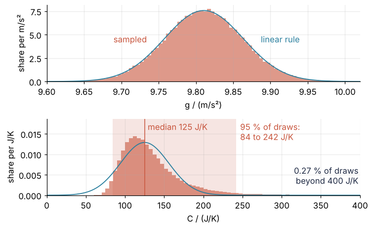
Histograms of 100,000 sampled results under the linear rule's normal curve. Top: g in m/s², the two coincide. Bottom: heat capacity C in J/K, the samples peak near 110 J/K with a long tail to the right, the curve reaches below every positive draw, and a line marks the median, 125 J/K, inside the 95 % interval of 84 to 242 J/K.

inside 0 to 400 J/K: 99.73 %   beyond 400 J/K: 0.27 %   negative: 2 of 100,000 draws
above 200 J/K: 6.5 %   smallest positive draw: 58 J/K

The bars for C hold 99.73 % of the draws; 0.27 % lie beyond 400 J/K, and the last two in 100,000 are negative, from ΔT draws below zero. In the bottom panel the bars peak near 110 J/K, left of the median, and trail off past 300 J/K. The linear curve reaches down to 50 J/K, below the smallest positive draw of 58 J/K, and has next to nothing above 200 J/K, where 6.5 % of the draws are.

Pitfalls

A normal input that must stay positive. The symptom is an sd that jumps between seeds, with a few negative values of a quantity that cannot be negative. The cause: a normal distribution puts about three draws in 100,000 more than four standard deviations below its mean, and for a ΔT of 0.40 ± 0.099 K that is below zero. When an input you draw directly cannot be negative, such as a mass or a ΔT read off a differential thermocouple, draw it from a log-normal, whose logarithm is normal, so every draw is positive. Matched to a mean m and a standard deviation σ, that is rng.lognormal(mu, s, N) with s² = ln(1 + (σ/m)²) and μ = ln m − s²/2. Step 5 shows the symptom without making the mistake. Its ΔT is the difference of two readings that each scatter by 0.07 K, and such readings can come out in the wrong order, so the negative draws belong to the claim about the thermometer. For the calorimeter as built in Step 4, report 84 to 242 J/K. A log-normal ΔT, with C's sd at 33 J/K and an interval of 80 to 207 J/K, would describe a different instrument.

An uncertainty that is not a standard deviation. The symptom is an interval too wide or too narrow by a factor of about two. The cause is an input quoted as half a scale division or a 95 % interval and passed to normal as a standard deviation. Convert first. A reading limited by a resolution d lies anywhere in a window of width d with equal probability, a standard uncertainty of d/√12: 0.1 K divisions give 0.029 K, not the 0.05 K of half a division. Or draw it with rng.uniform(x - d/2, x + d/2, N). A 95 % interval is about ± 2 standard deviations.

Too few draws for the interval. At N = 1,000 the upper end of C's 95 % interval moves from 224 to 259 J/K over seeds 1 to 5, against 241 to 244 J/K at N = 100,000. The 97.5th percentile is decided by the 25 largest of 1,000 draws. Use 100,000, a few milliseconds for the calorimeter, and rerun with a second seed: if a digit you report moves, N is too small.

Variations

Inputs quoted with a correlation coefficient. An error budget may give a correlation coefficient ρ instead of the shared source. For the two readings of Step 4 it is the share of each reading's variance that comes from the shared offset, 0.3²/(0.3² + 0.07²) = 0.95. Draw both inputs at once with rng.multivariate_normal([m1, m2], [[s1**2, rho*s1*s2], [rho*s1*s2, s2**2]], N), where s1 and s2 are each reading's total sd, √(0.07² + 0.3²) = 0.31 K, not the 0.07 K of its own scatter.
Parameters from a fit. To propagate a quantity derived from fitted parameters, a half-life from a decay rate for example, draw the parameters with rng.multivariate_normal(popt, pcov, N) from the output of curve_fit, as in curve_fit from the ground up.
A formula that does not take arrays. A root finder or an if inside the formula breaks the array call. Wrap it in np.vectorize or loop over the draws; propagate and linear_rule stay as they are.
Linear propagation without the gradient code. The uncertainties package carries values with their σ through arithmetic and applies the linear rule as it goes, correlations included: ufloat(50, 0.5) / ufloat(0.40, 0.099) gives 125 ± 31, the linear rule's answer in Step 5.

Cheat sheet

rng = np.random.default_rng(1)                       # seed once, draw in a fixed order
x = rng.normal(value, sigma, N)                      # one input; sigma is a standard uncertainty
inputs = {"T1": (22.10, 0.07), "c": (0.0, 0.3)}      # a shared error source is an input of its own
y = f(**{k: rng.normal(v, s, N) for k, (v, s) in inputs.items()})   # formula on arrays
y.mean(), y.std(ddof=1)                              # report these if mean = median, symmetric
np.median(y), np.percentile(y, [2.5, 97.5])          # otherwise these: median, 95 % interval
slope_i = (f(x_i + h) - f(x_i - h)) / (2 * h)        # central difference, h = sigma_i / 1000
sigma_f = np.sqrt(sum((slope_i * sigma_i) ** 2))     # linear rule, independent inputs