The Kalman filter: a battery's charge from a drifting current and noisy voltage (Python)

The question

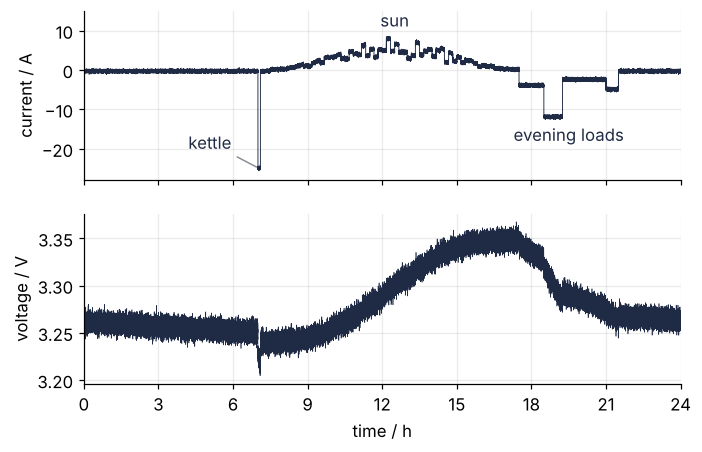
A home storage battery has to report its state of charge every second, and it has two witnesses for it, both flawed. Take one 50 Ah lithium iron phosphate cell standing in for the pack, through one day: standby at night, a kettle at 7:00, charging from the roof between 7:30 and 17:30 under passing clouds, household loads in the evening. Here are the current and the voltage its management system measures, one reading per second:

Show code

import numpy as np
import matplotlib.pyplot as plt

plt.rcParams.update({
    "figure.figsize": (7, 3.6), "figure.dpi": 110,
    "axes.spines.top": False, "axes.spines.right": False,
    "axes.grid": True, "grid.alpha": 0.25,
    "font.size": 11, "lines.linewidth": 1.8,
})
INK, ACCENT, SECOND, MUTED = "#1f2a44", "#c8553d", "#2a7f9e", "#8a8f98"

# Illustrative values for one LFP cell. The data are synthetic so that the truth is known;
# pretend you have not seen this cell.
CAPACITY_AH, DT = 50.0, 1.0                  # Ah, s
V0, K_OCV, R0_OHM = 3.20, 0.20, 1.0e-3       # V, V per unit charge (2 mV per percent), ohm
OFFSET_A, SIGMA_I, SIGMA_V = 0.10, 0.2, 5e-3 # current sensor offset and noise in A, voltage noise in V
SOC0, N = 0.31, 86_400                       # true charge at midnight, readings in a day

rng = np.random.default_rng(220)
t = np.arange(1, N + 1) * DT                 # time of each reading, s
hour = (t - DT) / 3600                       # start of the second the current flows in, h

# True current, positive when charging, in A; the draws come in a fixed order: clouds, current, voltage
clouds = rng.uniform(0.35, 1.0, 144)         # one factor per 10 minutes
I = np.full(N, -0.4)                         # standby
I[(hour >= 7.0) & (hour < 7.1)] = -25.0      # kettle
sun = (hour >= 7.5) & (hour < 17.5)
I[sun] = 8.0 * np.sin(np.pi * (hour[sun] - 7.5) / 10) ** 2 * clouds[(hour[sun] * 6).astype(int)]
for start, stop, amps in [(17.5, 18.5, -4.0), (18.5, 19.25, -12.0), (19.25, 21.0, -2.5), (21.0, 21.5, -5.0)]:
    I[(hour >= start) & (hour < stop)] = amps

c = DT / (3600 * CAPACITY_AH)                # charge fraction one ampere adds in one step
soc = SOC0 + c * np.cumsum(I)
I_m = I + OFFSET_A + SIGMA_I * rng.standard_normal(N)
V = V0 + K_OCV * soc + R0_OHM * I + SIGMA_V * rng.standard_normal(N)

# The two witnesses on their own
soc_count = SOC0 + c * np.cumsum(I_m)        # counting, started from the true charge (its best case)
soc_volt = (V - V0) / K_OCV                  # the curve, read naively
soc_volt_r = (V - V0 - R0_OHM * I_m) / K_OCV # the curve after subtracting the resistance drop


def rms(err):
    return 100 * np.sqrt(np.mean(err ** 2))


fig, (ax1, ax2) = plt.subplots(2, 1, figsize=(7, 4.4), sharex=True)
ax1.plot(t / 3600, I_m, color=INK, lw=0.6)
ax1.set(ylabel="current / A", ylim=(-28, 15), yticks=[-20, -10, 0, 10])
ax1.annotate("kettle", (7.05, -25), xytext=(4.2, -20), color=INK,
             arrowprops=dict(arrowstyle="-", color=MUTED, lw=1))
ax1.text(12.5, 10, "sun", ha="center", va="bottom", color=INK)
ax1.text(19.5, -18, "evening loads", ha="center", color=INK)
ax2.plot(t / 3600, V, color=INK, lw=0.4)
ax2.set(xlabel="time / h", ylabel="voltage / V", xlim=(0, 24), xticks=range(0, 25, 3))
plt.show()

print(f"true charge over the day       {100 * soc.min():5.1f} % to {100 * soc.max():.1f} %")
print(f"offset counted by midnight     {OFFSET_A * N * DT / 3600:5.2f} Ah")
print(f"counting                       off by {100 * (soc_count[-1] - soc[-1]):+.2f} % at midnight, "
      f"RMS {rms(soc_count - soc):.2f} %")
print(f"kettle's voltage shift         {1e3 * 25 * R0_OHM:5.1f} mV, read as {100 * 25 * R0_OHM / K_OCV:.1f} % of charge")
print(f"voltage alone                  RMS {rms(soc_volt - soc):.2f} %, largest error {100 * np.abs(soc_volt - soc).max():.1f} %")
print(f"voltage minus R0 I             RMS {rms(soc_volt_r - soc):.2f} %")

Measured current in A and measured cell voltage in V over 24 hours. The current dips to -25 A for the kettle at 7:00, rises in a cloudy hump up to about 8 A while the sun charges the cell, and steps down through the evening loads. The voltage follows the same jumps on top of a slow rise and fall.

true charge over the day        20.1 % to 73.6 %
offset counted by midnight      2.40 Ah
counting                       off by +4.77 % at midnight, RMS 2.75 %
kettle's voltage shift          25.0 mV, read as 12.5 % of charge
voltage alone                  RMS 3.11 %, largest error 18.8 %
voltage minus R0 I             RMS 2.51 %

The first witness is the current. Add up amperes times seconds and the charge comes out smooth, which is called coulomb counting. But this current sensor reads 0.1 A too high, an error that never averages away: by midnight counting has added 2.40 Ah that never flowed and is off by 4.77 % of the cell, although it started from the true charge.

The second witness is the voltage. The open-circuit voltage of a cell rises with its charge, so the charge can be read off a curve. For this chemistry the curve is flat, 2 mV per percent of charge, and 5 mV of voltmeter noise become 2.5 % of charge on every reading. The voltage also carries the drop across the internal resistance, so every change of load shifts it: the kettle's 25 A move it by 25.0 mV, which the curve reads as 12.5 % of charge. Read naively, the voltage is off by 3.11 % RMS, with jumps up to 18.8 %. Subtracting the resistance drop removes the jumps and keeps the noise, 2.51 % RMS.

So both witnesses are right about something. Counting is precise from one second to the next and wrong over hours; the voltage is right on average and wrong on every single reading. The question is how to combine them, second by second, and how much each should count at a given moment. The Kalman filter answers it with a weighting by variances that is recomputed at every reading and changes along the day.

The idea: multiply what you expect by what you measure

Start from the estimate one second ago and move it forward by the counted current. That is the prediction, and it is not a single number but a bell curve: a mean, the best guess, and a width, how far off the guess may be. The counted current is itself noisy, so each step forward widens the bell; the variance that each prediction step adds is called \(q\). The measurement is the voltage, with the resistance drop subtracted and turned into charge through the curve: a second bell, centered on whatever the reading says and 2.5 % wide. The new estimate is the product of the two bells.

The product is not an arbitrary choice. For each candidate charge, ask how plausible it is given the prediction, and how plausible given the voltage. The current sensor and the voltmeter make their errors independently, so the plausibility of that charge given both witnesses is the product of the two. The product of two bells is again a bell, narrower than both: its inverse variance is the sum of the two inverse variances, \(1/\sigma^2 = 1/\sigma_-^2 + 1/\sigma_z^2\), with \(\sigma_-\) the width of the prediction and \(\sigma_z\) that of the measurement. Its mean is the average of the two means, each weighted by its own inverse variance, \(1/\sigma_-^2\) and \(1/\sigma_z^2\), so it sits closer to the narrower bell. With \(n\) readings of equal width this is the plain mean, with the width \(\sigma/\sqrt n\) of The standard error of the mean; the standard error is the special case in which every witness is equally good.

How far the estimate moves, as a fraction of the way from prediction to measurement, is called the gain, \(K = \sigma_-^2/(\sigma_-^2 + \sigma_z^2)\). A gain of 1 means trust the voltage, a gain of 0 means trust the counting.

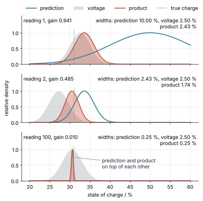
At midnight the system wakes up knowing nothing better than 50 ± 10 %. Here are prediction, measurement, and product at the first, the second, and the hundredth reading, each curve scaled to a peak of 1 so that the widths can be compared:

Show code

def predict(x, P, u, q):
    return x + c * u, P + q


def update(x, P, z, r):
    K = P / (P + r)
    return x + K * (z - x), (1 - K) * P, K


q = (SIGMA_I * c) ** 2                       # what the counted current's noise adds per step
r = (SIGMA_V / K_OCV) ** 2                   # one voltage reading, in charge units
x, P = 0.5, 0.1 ** 2                         # the wake-up guess: 50 +- 10 %
keep = {}
for k in range(1000):
    x_pred, P_pred = predict(x, P, I_m[k], q)
    x, P, K = update(x_pred, P_pred, soc_volt_r[k], r)
    keep[k + 1] = (x_pred, P_pred, soc_volt_r[k], x, P, K)

soc_grid = np.linspace(20, 60, 4000)
bell = lambda mean, var: np.exp(-0.5 * (soc_grid - 100 * mean) ** 2 / (1e4 * var))

fig, axes = plt.subplots(3, 1, figsize=(7, 6.6), sharex=True)
for ax, n in zip(axes, [1, 2, 100]):
    x_pred, P_pred, z, x, P, K = keep[n]
    ax.axvline(100 * soc[n - 1], ymax=1.1 / 1.55, color=MUTED, lw=1, ls="--", label="true charge")   # stops below the text
    ax.plot(soc_grid, bell(x_pred, P_pred), color=SECOND, label="prediction")
    ax.fill_between(soc_grid, bell(z, r), color=MUTED, alpha=0.3, lw=0, label="voltage")
    ax.fill_between(soc_grid, bell(x, P), color=ACCENT, alpha=0.35, lw=0)
    ax.plot(soc_grid, bell(x, P), color=ACCENT, label="product")
    ax.text(0.01, 0.96, f"reading {n}, gain {K:.3f}", transform=ax.transAxes, ha="left", va="top")
    ax.text(0.99, 0.96, f"widths: prediction {100 * np.sqrt(P_pred):.2f} %, voltage {100 * np.sqrt(r):.2f} %\n"
            f"product {100 * np.sqrt(P):.2f} %", transform=ax.transAxes, ha="right", va="top")
    ax.set(ylim=(0, 1.55), yticks=[0, 0.5, 1])
axes[2].annotate("prediction and product\non top of each other", (100 * keep[100][3] + 0.3, 0.75),
                 xytext=(38, 0.55), va="center", color=INK,
                 arrowprops=dict(arrowstyle="-", color=MUTED, lw=1))
handles, labels = axes[0].get_legend_handles_labels()
order = [1, 2, 3, 0]                         # prediction, voltage, product as in the widths, then true charge
axes[0].legend([handles[i] for i in order], [labels[i] for i in order], frameon=False,
               loc="lower left", bbox_to_anchor=(0, 1.0), ncol=4)
axes[1].set_ylabel("relative density")
axes[-1].set_xlabel("state of charge / %")
plt.show()

print("reading   prediction width   voltage width     gain   product width")
for n in [1, 2, 100, 1000]:
    x_pred, P_pred, z, x, P, K = keep[n]
    print(f"{n:7d}   {100 * np.sqrt(P_pred):14.2f} %   {100 * np.sqrt(r):11.2f} %   {K:6.3f}   {100 * np.sqrt(P):11.2f} %")
print(f"widening of the prediction per second at reading 100: {q / (2 * keep[100][4]):.1e} of its width")

Relative density against state of charge in %, at readings 1, 2, and 100. Blue: prediction. Gray fill: voltage reading. Red: their product. Dashed gray: true charge. At reading 1 the product sits on the reading, gain 0.941; at reading 2 halfway, gain 0.485; at reading 100 on the narrow prediction, gain 0.010.

reading   prediction width   voltage width     gain   product width
      1            10.00 %          2.50 %    0.941          2.43 %
      2             2.43 %          2.50 %    0.485          1.74 %
    100             0.25 %          2.50 %    0.010          0.25 %
   1000             0.08 %          2.50 %    0.001          0.08 %
widening of the prediction per second at reading 100: 9.9e-08 of its width

At the first reading the prediction is 10 % wide and the voltage 2.5 %, the gain is 0.941, and the product sits almost on the measurement. At the second, the prediction has narrowed to 2.43 %, about as wide as the measurement, the gain is 0.485, and the product lands halfway between them. By the hundredth reading the prediction is 0.25 % wide and the gain 0.010: the voltage moves the estimate by a hundredth of its disagreement. The voltage did not get worse. The prediction got better, because it carries every reading before it.

Between readings the prediction widens by \(q\), but at one reading per second that is about a part in ten million of its width (\(9.9 \times 10^{-8}\) at the hundredth reading), far too little to see. The animation prints the widths as numbers instead:

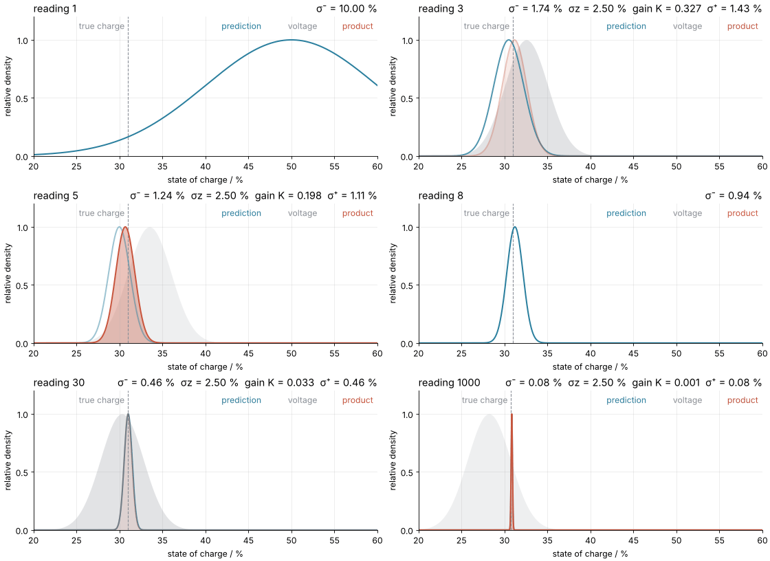
The filter waking up at midnight, reading by reading: the blue prediction, the gray voltage reading, and the red product forming between them. The product narrows and settles onto the prediction while the printed gain falls from 0.941 at reading 1 to 0.001 at reading 1000.

How I built this: each reading is drawn in three held states with Matplotlib's FuncAnimation, the technique of Matplotlib animation with FuncAnimation: a probe sweep as a small GIF; the source is animations/kalman-update/scene.py.

After a thousand readings the gain is 0.001, and a reading moves the estimate by a thousandth of its disagreement with the prediction. The filter has become nearly deaf to the voltage. That is right only if the prediction really is as good as its width claims, and counting with a sensor that reads 0.1 A too high is not.

Formalization

Here are the idea's two steps in symbols, with \(\hat x\) the estimate of the state, the quantity tracked (here the charge), \(u\) the counted current, \(z\) the measurement in charge units, and \(c\) the fraction of the capacity one ampere fills in one step:

\[ \text{predict:}\quad \hat x^- = \hat x + c\,u, \qquad P^- = P + q, \qquad\qquad \text{update:}\quad K = \frac{P^-}{P^- + r}, \qquad \hat x = \hat x^- + K\,(z - \hat x^-), \qquad P = (1 - K)\,P^- . \]

\(P\) is the variance of the estimate's error, the squared width of the bell, so \(P^- = \sigma_-^2\) and \(r = \sigma_z^2\). When the state has more than one entry, the same two steps read

\[ \hat x^- = F\hat x + Bu, \qquad P^- = FPF^\top + Q, \qquad K = P^-H^\top\left(HP^-H^\top + R\right)^{-1}, \qquad \hat x = \hat x^- + K\,(z - H\hat x^-), \qquad P = (I - KH)\,P^- . \]

\(F\) moves the state one step forward, \(B\) adds the input, and \(H\) says what the meter would read for a given state. \(HP^-H^\top\) is then the prediction's variance in the meter's units and \(R\) the measurement's covariance, so with one state entry and \(H = 1\) the gain is the scalar one above.

\(P\) is now the covariance matrix of the estimate's errors: on its diagonal the variance of each state entry, off it how the errors of two entries move together, positive when one being too high tends to come with the other too high, zero when they are unrelated. \(FPF^\top\) moves the errors along with the state, and \(Q\) adds the variance of new, independent errors. While \(P\) is diagonal, this is the linear rule of uncertainty propagation. When \(F\) mixes two state entries it also fills the off-diagonal entries, which that rule has no place for.

The gain is a ratio of variances, and without process noise the filter is an average. With \(q\) near zero, the gain at reading \(n\) is close to \(1/n\), the weight a running mean gives its \(n\)-th reading: 0.010 at the hundredth, 0.001 at the thousandth.

A filter is only as honest as its \(q\). Here is the one-state filter run over the day, with \(q\) from the current sensor's noise alone, \(1.2 \times 10^{-12}\) per second:

Show code

def scalar_filter(q):
    x, P = 0.5, 0.1 ** 2
    xs, Ps, Ks = np.empty(N), np.empty(N), np.empty(N)
    for k in range(N):
        x, P = predict(x, P, I_m[k], q)
        x, P, Ks[k] = update(x, P, soc_volt_r[k], r)
        xs[k], Ps[k] = x, P
    return xs, Ps, Ks


soc_1, P_1, K_1 = scalar_filter(q)
err_1 = 100 * (soc_1 - soc)
print(f"q                         {q:.1e} per second")
print(f"gain at midnight          {K_1[-1]:.1e}, so a memory of 1/K = {1 / K_1[-1] * DT / 3600:.1f} h")
print(f"reported width            {100 * np.sqrt(P_1[-1]):.3f} %")
print(f"error at midnight         {err_1[-1]:+.2f} %")
print(f"RMS error over the day    {rms(soc_1 - soc):.2f} %")
soc_9, _, _ = scalar_filter(1e-9)
print(f"same with q = 1e-9        RMS {rms(soc_9 - soc):.2f} %")

fig, ax = plt.subplots(figsize=(7, 3.4))
ax.axhline(0, color=MUTED, lw=1)
err_count = 100 * (soc_count - soc)
ax.plot(t / 3600, err_count, color=SECOND)
ax.text(23.8, err_count[-1] + 0.3, "counting", ha="right", va="bottom", color=SECOND)
band = 200 * np.sqrt(P_1)
ax.fill_between(t / 3600, err_1 - band, err_1 + band, color=ACCENT, alpha=0.15, lw=0)
ax.plot(t / 3600, err_1, color=ACCENT)
ax.text(23.8, err_1[-1] + 0.35, f"one-state filter\nreported width {100 * np.sqrt(P_1[-1]):.3f} %\noff by {err_1[-1]:.2f} %",
        ha="right", va="bottom", color=ACCENT)
ax.set(xlabel="time / h", ylabel="error / %", xlim=(0, 24), ylim=(-3, 6), xticks=range(0, 25, 3))
plt.show()

q                         1.2e-12 per second
gain at midnight          4.4e-05, so a memory of 1/K = 6.2 h
reported width            0.017 %
error at midnight         +1.15 %
RMS error over the day    0.84 %
same with q = 1e-9        RMS 0.06 %

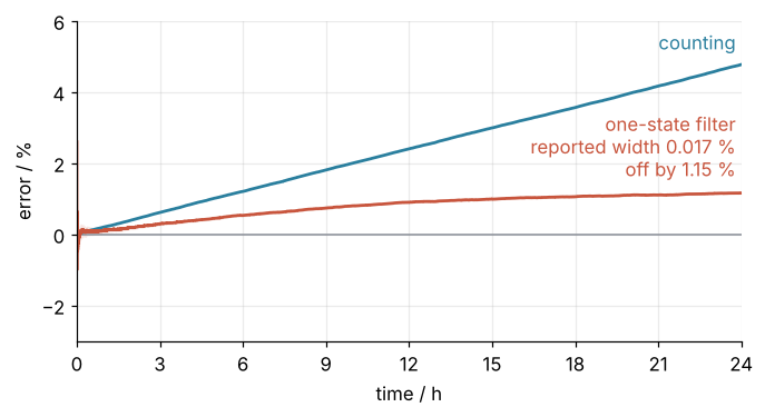
Error of the estimated state of charge in % over 24 hours. Blue: counting alone, drifting up to about 4.8 %. Red: the one-state filter with its own 2-sigma band, which is too thin to see; the error wanders away from zero and ends at about 1.2 % at midnight.

The gain falls to \(4.4 \times 10^{-5}\), so the filter remembers about \(1/K\) readings, 6.2 hours of them. It reports a width of 0.017 % and is off by 1.15 % at midnight, 0.84 % RMS: sure and wrong, because the offset is not noise. Raising \(q\) by hand to \(10^{-9}\) brings the RMS to 0.06 %, but the filter then knows only that something drifts, not what.

Put the offset into the state and the drift disappears. Make the offset \(b\) a second state entry, \(x = (\text{SOC}, b)\), measure \(z = V - V_0 - R_0 I_m\) in volts, and the battery's model is

\[ F = \begin{pmatrix} 1 & -c \\ 0 & 1 \end{pmatrix}, \quad B = \begin{pmatrix} c \\ 0 \end{pmatrix}, \quad H = \begin{pmatrix} k & -R_0 \end{pmatrix}, \quad Q = \begin{pmatrix} (0.2\ \text{A}\cdot c)^2 & 0 \\ 0 & 0 \end{pmatrix}, \quad R = (5\ \text{mV})^2, \]

with \(k\) the slope of the curve, 0.20 V per unit charge. The counted current \(I_m\) is the true current plus \(b\), so one step of counting adds \(c\,I_m\) and must take back \(c\,b\), which is the \(-c\) in \(F\). The offset itself stays as it was, the 0 and 1 of the second row, and its 0 in \(Q\) says it is assumed constant. The voltmeter sees \(k\) times the charge plus \(R_0\) times the true current, and since \(z\) subtracts \(R_0 I_m = R_0 (I + b)\), an offset leaves \(-R_0 b\) in the reading, which is the \(-R_0\) in \(H\). The filter starts from 50 ± 10 % and an offset of 0 ± 0.2 A:

Show code

def kalman(x, P, F, B, H, Q, R, u, z):
    """The five equations, once per reading; returns the estimates and their covariances."""
    xs, Ps = np.empty((len(z), len(x))), np.empty((len(z), len(x), len(x)))
    for k in range(len(z)):
        x, P = F @ x + B * u[k], F @ P @ F.T + Q                       # predict
        S = H @ P @ H.T + R
        K = np.linalg.solve(S, H @ P).T                                # P H^T S^-1 without an inverse
        x, P = x + K @ (z[k] - H @ x), (np.eye(len(x)) - K @ H) @ P    # update
        xs[k], Ps[k] = x, P
    return xs, Ps


F = np.array([[1.0, -c], [0.0, 1.0]])
B = np.array([c, 0.0])
H = np.array([[K_OCV, -R0_OHM]])
Q = np.diag([(SIGMA_I * c) ** 2, 0.0])
R = np.array([[SIGMA_V ** 2]])
z = (V - V0 - R0_OHM * I_m)[:, None]
xs, Ps = kalman(np.array([0.5, 0.0]), np.diag([0.1 ** 2, 0.2 ** 2]), F, B, H, Q, R, I_m, z)

b_hat, b_sd = xs[:, 1], np.sqrt(Ps[:, 1, 1])
corr = Ps[:, 0, 1] / np.sqrt(Ps[:, 0, 0] * Ps[:, 1, 1])
print("after    offset estimate      correlation of charge and offset errors")
for h in [1, 4, 24]:
    k = int(h * 3600 / DT) - 1
    print(f"{h:3d} h    {b_hat[k]:.3f} ± {b_sd[k]:.3f} A    {corr[k]:+.2f}")
print(f"the true offset in one reading: {1e3 * R0_OHM * OFFSET_A:.1f} mV, against {1e3 * SIGMA_V:.0f} mV of noise")

fig, ax = plt.subplots(figsize=(7, 3.4))
ax.axhline(OFFSET_A, color=MUTED, lw=1, ls="--")
ax.fill_between(t / 3600, b_hat - 2 * b_sd, b_hat + 2 * b_sd, color=ACCENT, alpha=0.15, lw=0)
ax.plot(t / 3600, b_hat, color=ACCENT)
ax.text(23.8, OFFSET_A + 0.02, "true offset 0.1 A", ha="right", va="bottom", color=MUTED)
ax.set(xlabel="time / h", ylabel="offset / A", xlim=(0, 24), ylim=(-0.3, 0.5), xticks=range(0, 25, 3))
plt.show()

after    offset estimate      correlation of charge and offset errors
  1 h    0.095 ± 0.068 A    -0.63
  4 h    0.113 ± 0.009 A    -0.81
 24 h    0.099 ± 0.001 A    -0.55
the true offset in one reading: 0.1 mV, against 5 mV of noise

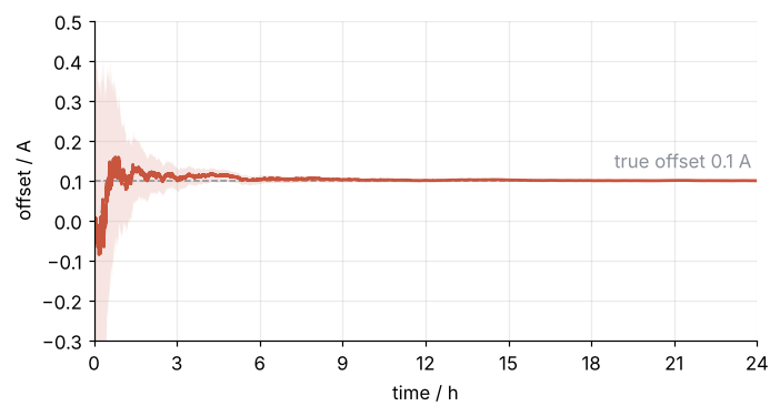
Estimated current sensor offset in A over 24 hours, with its 2-sigma band, and the true offset of 0.1 A dashed. The estimate starts at 0 with a wide band, finds 0.1 A within the first hours, and the band closes onto the dashed line.

After one hour the filter has the offset at 0.095 ± 0.068 A, after four at 0.113 ± 0.009 A, and at midnight at 0.099 ± 0.001 A. A reading carries the offset only as \(-R_0 b\), 0.1 mV against 5 mV of noise, so the filter learns it mostly through \(P\). \(P\) starts diagonal, but multiplying out \(FPF^\top\) with the \(-c\) in \(F\) adds \(-c\) times the offset's variance to the off-diagonal entry every second. Counting takes away \(c\) times the estimated offset, so an offset estimated too high comes with a charge estimated too low, and the reading, which sees both, couples them as well.

Their correlation, the off-diagonal entry over the product of the two widths, is −0.63 after 1 h and −0.81 after 4 h. The offset entry of \(K\) soon comes mostly from that off-diagonal entry, and it is negative: a reading lower than predicted lowers the charge and raises the offset, because counting must have added too much. By midnight the correlation has relaxed to −0.55. The offset is pinned down by then, so most of the charge's remaining error is fresh current noise, unrelated to the offset.

See it in code

There is no library function to call here: the filter is the five equations above, about 15 lines of NumPy in the hidden cells, and the same function runs the battery's whole day. Here are the three estimates against the truth:

Show code

soc_kf = xs[:, 0]
print("estimate          RMS error   error at midnight")
for name, est in [("counting", soc_count), ("voltage alone", soc_volt), ("Kalman filter", soc_kf)]:
    print(f"{name:15s}   {rms(est - soc):7.2f} %   {100 * (est[-1] - soc[-1]):+13.2f} %")
print(f"largest filter error after the first minute: {100 * np.abs(soc_kf - soc)[60:].max():.2f} % "
      f"(at {t[60:][np.argmax(np.abs(soc_kf - soc)[60:])]:.0f} s)")

fig, (ax1, ax2) = plt.subplots(2, 1, figsize=(7, 4.6), sharex=True)
hours = t / 3600
ax1.plot(hours, 100 * soc_volt, color=MUTED, lw=0.3, alpha=0.45, label="voltage alone")
ax1.plot(hours, 100 * soc, color=INK, lw=3.2, label="truth")
ax1.plot(hours, 100 * soc_count, color=SECOND, label="counting")
ax1.plot(hours, 100 * soc_kf, color=ACCENT, lw=1.4, label="Kalman filter")
ax1.set(ylabel="charge / %", ylim=(10, 90))
handles, labels = ax1.get_legend_handles_labels()
order = [1, 2, 3, 0]                                     # truth, counting, filter, voltage alone
leg = ax1.legend([handles[i] for i in order], [labels[i] for i in order], frameon=False,
                 loc="lower left", bbox_to_anchor=(0, 1.0), ncol=4, handlelength=1.6, columnspacing=1.2)
leg.get_lines()[3].set(alpha=1, linewidth=1.8)          # the voltage key readable, not a hairline
ax2.plot(hours, 100 * (soc_volt - soc), color=MUTED, lw=0.3, alpha=0.45)
ax2.plot(hours, 100 * (soc_count - soc), color=SECOND)
ax2.plot(hours, 100 * (soc_kf - soc), color=ACCENT)
for x_text, ha, name, est, color in [(0.2, "left", "RMS: voltage alone", soc_volt, MUTED),
                                     (12.6, "center", "counting", soc_count, SECOND),
                                     (23.8, "right", "Kalman filter", soc_kf, ACCENT)]:
    ax2.text(x_text, 14.5, f"{name} {rms(est - soc):.2f} %", ha=ha, va="center", color=color)
ax2.set(xlabel="time / h", ylabel="error / %", xlim=(0, 24), ylim=(-16, 17), xticks=range(0, 25, 3))
plt.show()

estimate          RMS error   error at midnight
counting             2.75 %           +4.77 %
voltage alone        3.11 %           +1.85 %
Kalman filter        0.03 %           +0.02 %
largest filter error after the first minute: 0.47 % (at 65 s)

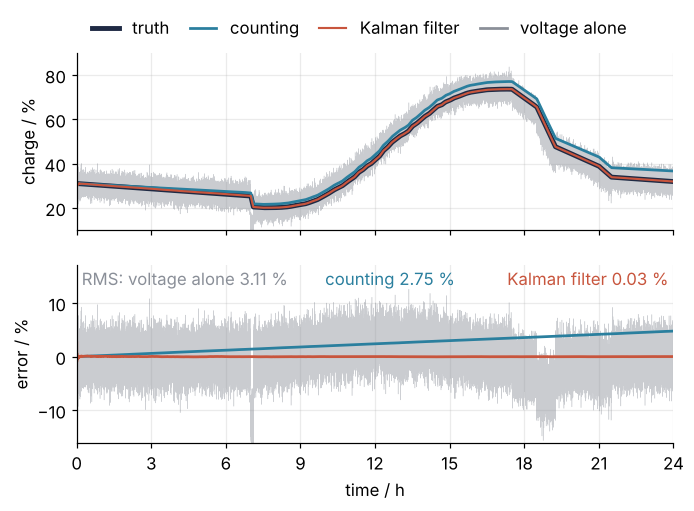
Top: state of charge in % over 24 hours; the truth, counting, the voltage alone as a noisy gray band, and the Kalman filter, which lies on the truth. Bottom: estimate minus truth in %; counting drifts to about 4.8 %, the voltage alone scatters by several percent, the filter stays at zero.

Counting is off by 2.75 % RMS, the voltage alone by 3.11 %, the filter by 0.03 %, nearly a hundred times closer than either witness on its own. After its first minute the filter's error never exceeds 0.47 %, and that worst moment comes at 65 s, while the offset is still unknown. This precision rests on a model that is exactly right: the curve here is a straight line, and \(R_0\) and the capacity are known because the data were made with them. A real cell's open-circuit curve is bent and moves with temperature, which is why battery management systems run the extended Kalman filter.

Where it shows up

The battery is one instance of a pattern that runs through engineering and the sciences: a model that predicts how a state moves, and a measurement that sees part of the state through noise.

Battery management. The extended Kalman filter linearizes the cell's full, curved open-circuit voltage at each step and estimates the charge together with the voltages across the cell's internal time constants. Gregory Plett's equivalent-circuit filters for electric vehicle packs are the standard reference.
Navigation. The Apollo guidance computer navigated to the Moon with a Kalman filter, after Stanley Schmidt at NASA Ames extended it to nonlinear orbits. A GPS receiver in a car or a drone fuses smooth but drifting inertial sensors with noisy but non-drifting satellite fixes, the battery's two witnesses again.
Particle physics. Detectors at CERN fit the tracks of charged particles with a Kalman filter: the state is position, direction, and the curvature in the magnetic field that gives the momentum, the prediction carries the track through the field and the material, and multiple scattering in that material is the process noise. Each detector layer the particle crosses is one measurement.
Weather and climate. Data assimilation corrects a running forecast model with millions of observations. The ensemble Kalman filter represents \(P\) by an ensemble of model runs, because the state has hundreds of millions of entries and \(P\) would have their square.
Neuroscience. Brain-computer interfaces decode intended movement from recordings of motor cortex neurons. The state is the velocity of the hand or a cursor, and the firing rates are the measurement.
Chemical engineering. A reactor's concentrations are estimated from a temperature measured every second and a concentration analyzed every few minutes. The model carries the estimate through the gaps, and each analysis corrects it.

In every case two things carry over: each step weighs prediction against measurement by their variances, and a quantity you do not know but expect to be constant, such as an offset or a drift, can be put into the state and learned.

The question

The idea: multiply what you expect by what you measure

Formalization

See it in code

Where it shows up

Further reading