Minimization with Optim.jl: the shape of a seven-atom cluster

The problem: the shape of seven argon atoms

Cool seven argon atoms until they stop moving, and they settle into a pentagonal bipyramid: five atoms in a ring, a sixth on top, a seventh underneath, −16.505 ε in all. With Optim.jl that shape takes one call to optimize. In practice it takes fifty, since a single call most often stops at −15.533 ε.

Each pair of atoms at distance \(r\) interacts through the Lennard-Jones potential

\[V(r) = 4\varepsilon\left[\left(\frac{\sigma}{r}\right)^{12} - \left(\frac{\sigma}{r}\right)^{6}\right],\]

whose well, \(\varepsilon\) deep, lies at \(r = 2^{1/6}\sigma\). All numbers below use \(\varepsilon = \sigma = 1\), reduced units; argon has \(\varepsilon/k_B \approx 120\) K and \(\sigma \approx 3.4\) Å. Summing \(V\) over the 21 pairs gives the cluster energy, which depends on 21 coordinates and has more than one minimum. A local minimizer goes downhill from its starting point until the ground is flat. Where it ends up is decided by the start, and by the method.

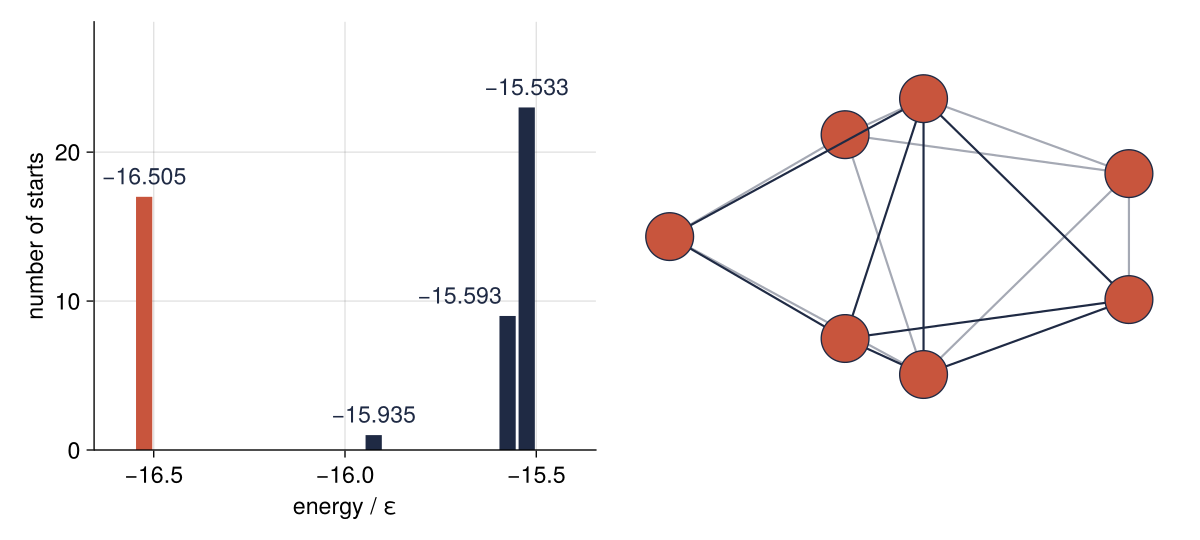
Left: how many of fifty random starts ended at each energy, in ε; the leftmost bar, at −16.505 ε, is the global minimum and not the tallest. Right: that structure, a pentagonal bipyramid, drawn without axes because the coordinates of a free cluster carry no meaning.

Behind the histogram are fifty starts, one optimize call each. Twenty-three stopped at −15.533 ε and seventeen found the bipyramid. Step 6 draws the figure.

Setup

Install the packages once with import Pkg; Pkg.add(["Optim", "ForwardDiff", "ADTypes", "CairoMakie"]); the other three ship with Julia. The first optimize call compiles for a few seconds, the later ones are fast. The only data are random atom positions, which random_start hands back as one flat vector, the form Optim moves.

using Optim, ForwardDiff, ADTypes, LinearAlgebra, Random, Printf, CairoMakie

const INK, ACCENT, SECOND, MUTED = "#1f2a44", "#c8553d", "#2a7f9e", "#8a8f98"
set_theme!(Theme(                          # the look of every figure below
    size = (880, 396), fontsize = 17,
    palette = (color = [INK, ACCENT, SECOND, MUTED],),
    Axis = (topspinevisible = false, rightspinevisible = false, xgridvisible = true, ygridvisible = true),
    Lines = (linewidth = 2.5,),
))

rng = Xoshiro(1)

# atoms closer than about 1 σ make the first step explode; see Pitfalls
function random_start(n; side = 2.5, d_min = 1.0)
    while true
        pos = side .* rand(rng, 3, n)          # one column per atom: x, y, z
        closest = minimum(norm(pos[:, i] - pos[:, j]) for i in 1:n-1 for j in i+1:n)
        # Optim moves one flat vector of 3n numbers; Step 1 shows how to get the atoms back
        closest > d_min && return vec(pos)
    end
end

@printf("pair distance at the bottom of the well: 2^(1/6) = %.5f σ\n", 2^(1 / 6))

pair distance at the bottom of the well: 2^(1/6) = 1.12246 σ

Step 1: Write the energy as a function of one flat vector

Optim changes the entries of a single vector; the physics wants a column per atom. reshape(x, 3, :) turns the vector into a 3 × n matrix that shares memory with x. Julia stores a matrix column by column, so \(x_1, y_1, z_1\) land in column 1, as they should. Write reshape(x, :, 3) and you get an n × 3 matrix whose rows mix coordinates of different atoms, and no error.

distances returns the \(n(n-1)/2\) pair distances, and the energy sums the potential over them. Nothing in either function fixes the number type to Float64; Step 3 shows why that matters.

function distances(x)
    pos = reshape(x, 3, :)
    n = size(pos, 2)
    return [norm(pos[:, i] - pos[:, j]) for i in 1:n-1 for j in i+1:n]
end

energy(x) = sum(r -> 4 * (r^-12 - r^-6), distances(x))

dimer = [0, 0, 0, 2^(1 / 6), 0, 0]
x0 = [0.0, 0.0, 0.0, 1.5, 0.0, 0.0, 0.3, 1.2, 0.0]    # three atoms, the start for Step 2
@printf("two atoms at 2^(1/6): E = %.6f ε\n", energy(dimer))
@printf("three atoms at x0:    E = %.6f ε\n", energy(x0))

two atoms at 2^(1/6): E = -1.000000 ε
three atoms at x0:    E = -1.285777 ε

Two atoms at the well's minimum give −1, as deep as the potential goes, so the code is correct. The three atoms of x0 have −1.286 ε, the value Step 2 starts from.

Step 2: Minimize three atoms and read the result

optimize takes the function, the start, and a method. Without a method it runs Nelder-Mead, which never looks at a slope, so name BFGS(): it steps against the gradient and, from how the gradient changes between steps, learns the curvature, the matrix of second derivatives known as the Hessian. The result is read through accessor functions:

res = optimize(energy, x0, BFGS())
println("minimum:    ", Optim.minimum(res))
println("minimizer:  ", round.(Optim.minimizer(res), digits = 4))
println("converged:  ", Optim.converged(res))
println("iterations: ", Optim.iterations(res))
println("f_calls:    ", Optim.f_calls(res))
println("g_calls:    ", Optim.g_calls(res))
println("g_residual: ", Optim.g_residual(res))

minimum:    -3.0
minimizer:  [0.1301, -0.0463, 0.0, 1.2215, 0.2162, 0.0, 0.4484, 1.0301, 0.0]
converged:  true
iterations: 16
f_calls:    42
g_calls:    42
g_residual: 6.154194850817358e-9

minimum is the final energy, −3.0. minimizer gives the coordinates where the run stopped, as flat as x0. iterations counts steps, f_calls and g_calls count evaluations of the energy and the gradient. g_residual is the biggest gradient component left at the end, 6.2e-9. Typing res alone prints a summary of all this plus the run time.

converged true means a stopping test passed, in practice that g_residual dropped below g_abstol, 1e-8 unless you pass Optim.Options(g_abstol = 1e-10) as the last argument of optimize. So the run ended on flat ground. Flat is not lowest, and it is not necessarily the cluster you had in mind; the pitfalls show both.

For three atoms, flat is also lowest, an equilateral triangle:

println(distances(Optim.minimizer(res)))

[1.1224620483200114, 1.1224620483518457, 1.1224620484326848]

The cost is the surprise. You gave no gradient, so Optim estimated each of the 42 gradients by central differences: two energy calls for each of the nine coordinates, 18 calls per gradient. f_calls does not count those: the run took about 800 energy calls, not 42.

Step 3: Supply the gradient

The chain rule gives the gradient of any pair sum. Moving atom \(i\) changes only its distances \(r_{ij}\) to the others, and \(\partial r_{ij}/\partial \mathbf r_i = (\mathbf r_i - \mathbf r_j)/r_{ij}\), so

\[\frac{\partial E}{\partial \mathbf r_i} = \sum_{j \ne i} \frac{V'(r_{ij})}{r_{ij}}\,(\mathbf r_i - \mathbf r_j), \qquad \frac{V'(r)}{r} = 24 r^{-8} - 48 r^{-14}.\]

Optim wants the gradient as gradient!(G, x): storage first, and the ! says the function writes into its first argument instead of returning a new vector. reshape(G, 3, :) shares memory with G, so writing into g fills G. The loop visits each pair once and adds the term to atom \(i\) and subtracts it from atom \(j\), Newton's third law.

ForwardDiff checks it. It runs energy itself on numbers that carry their derivatives along, so it returns the exact derivative of your code, not an estimate. That only works because energy accepts any number type.

function gradient!(G, x)
    fill!(G, 0)
    pos, g = reshape(x, 3, :), reshape(G, 3, :)
    n = size(pos, 2)
    for i in 1:n-1, j in i+1:n
        d = pos[:, i] - pos[:, j]
        r = norm(d)
        f = (24 * r^-8 - 48 * r^-14) .* d
        g[:, i] .+= f
        g[:, j] .-= f
    end
    return G
end

x5 = random_start(5)
G = zeros(15)
gradient!(G, x5)
G_ad = ForwardDiff.gradient(energy, x5)
@printf("largest difference to ForwardDiff: %.1e of the largest component\n", maximum(abs, G - G_ad) / maximum(abs, G_ad))

largest difference to ForwardDiff: 8.2e-16 of the largest component

A difference of 8.2e-16 is rounding, nothing more. Now five atoms from one start, three ways: without a gradient, with gradient!, and with automatic differentiation chosen by AutoForwardDiff(). ADTypes only names the backend, the package that computes the derivative; ForwardDiff does the work.

runs5 = [("finite differences", optimize(energy, x5, BFGS())),
         ("gradient!", optimize(energy, gradient!, x5, BFGS())),
         ("AutoForwardDiff()", optimize(energy, x5, BFGS(); autodiff = AutoForwardDiff()))]
for (label, r) in runs5
    @printf("%-18s  E = %.6f ε  converged = %-5s  f_calls = %4d  g_calls = %4d\n",
            label, Optim.minimum(r), Optim.converged(r), Optim.f_calls(r), Optim.g_calls(r))
end

finite differences  E = -9.103851 ε  converged = false  f_calls = 1703  g_calls = 1703
gradient!           E = -9.103852 ε  converged = true   f_calls =  117  g_calls =  117
AutoForwardDiff()   E = -9.103852 ε  converged = true   f_calls =  117  g_calls =  117

Both exact gradients reach −9.103852 ε in 117 calls, though each ForwardDiff call does more work than gradient!, which the counts do not show. Without one, BFGS ran into its limit of 1000 iterations one unit short in the sixth digit, after 1703 gradient estimates of 30 energy calls each, about 51,000 calls. Write the gradient when it is cheap to write and speed matters; take AutoForwardDiff() when it is not.

Five atoms should form a trigonal bipyramid, a triangle with one atom above and one below its center: nine bonds near 1.12 σ, and one long distance between the two tips, about 1.83 σ.

println(round.(sort(distances(Optim.minimizer(runs5[2][2]))), digits = 3))

[1.12, 1.12, 1.12, 1.12, 1.12, 1.12, 1.124, 1.124, 1.124, 1.826]

Step 4: Compare methods by their function evaluations

Seven atoms now, one start, five runs, three of them with methods you have not met. Nelder-Mead never computes a slope: it keeps 22 trial points (a simplex; in two variables it would be a triangle) and keeps moving the worst one. L-BFGS stores a handful of recent steps in place of the 21 × 21 curvature matrix, and conjugate gradient stores no matrix, choosing each direction from the gradient and the previous direction.

x7 = random_start(7)
runs7 = [("NelderMead()", optimize(energy, x7, NelderMead())),
         ("BFGS()", optimize(energy, x7, BFGS())),
         ("BFGS() + gradient!", optimize(energy, gradient!, x7, BFGS())),
         ("LBFGS() + gradient!", optimize(energy, gradient!, x7, LBFGS())),
         ("ConjugateGradient()", optimize(energy, gradient!, x7, ConjugateGradient()))]
for (label, r) in runs7
    @printf("%-20s  E = %10.6f ε  converged = %-5s  f_calls = %4d  g_calls = %3d\n",
            label, Optim.minimum(r), Optim.converged(r), Optim.f_calls(r), Optim.g_calls(r))
end

NelderMead()          E = -13.830411 ε  converged = false  f_calls = 1717  g_calls =   0
BFGS()                E = -15.935043 ε  converged = true   f_calls =  193  g_calls = 193
BFGS() + gradient!    E = -15.593211 ε  converged = true   f_calls =  190  g_calls = 190
LBFGS() + gradient!   E = -16.505384 ε  converged = true   f_calls =  113  g_calls = 113
ConjugateGradient()   E = -16.505384 ε  converged = true   f_calls =  130  g_calls =  81

Nelder-Mead ran out of iterations, 1000 in Optim, with converged false and an energy that is not a minimum. With 21 variables, function values alone are too little. BFGS without the gradient made 193 estimates of 42 energy calls each, over 8,000 calls, against 190 with gradient!.

Then look at where they landed. The two BFGS runs differ only in how the gradient is computed, and they end in different minima, −15.935 and −15.593 ε. L-BFGS and conjugate gradient reach −16.505 ε. Their paths from this start happened to lead there; every method here is local. One run, whatever the method, cannot tell you whether its minimum is the lowest.

Step 5: Start fifty times

The cure is many starts and the lowest result. Two runs in the same minimum are not equal bit for bit, so round to three decimals before counting:

results = [optimize(energy, gradient!, random_start(7), BFGS()) for _ in 1:50]
Es = Optim.minimum.(results)

println(count(Optim.converged, results), " of 50 converged")
for E in sort(unique(round.(Es, digits = 3)))
    @printf("E = %8.3f ε   %2d starts\n", E, count(e -> round(e, digits = 3) == E, Es))
end

50 of 50 converged
E =  -16.505 ε   17 starts
E =  -15.935 ε    1 starts
E =  -15.593 ε    9 starts
E =  -15.533 ε   23 starts

Four distinct values: seven Lennard-Jones atoms have four minima, and all of them turned up. −15.533 ε took 23 starts, the global minimum 17. The same recipe works for any function: draw starts over the whole region where a sensible answer can lie, here a box a few σ wide because bonds are about 1 σ, and add starts until the best value has turned up several times.

The energy says which minimum, not what it looks like, so count each atom's neighbors. In a pentagonal bipyramid each ring atom touches two ring neighbors and both tips, four in all, and each tip touches the five ring atoms and the other tip, six: 16 bonds. The diagonal of the distance matrix holds each atom's zero distance to itself, so it is set to Inf to keep an atom from counting itself.

best = argmin(Optim.minimum, results)
pos = reshape(Optim.minimizer(best), 3, :)
D = [norm(pos[:, i] - pos[:, j]) for i in 1:7, j in 1:7]
D[diagind(D)] .= Inf
bonded = D .< 1.3
nb = vec(sum(bonded, dims = 2))
@printf("E = %.6f ε\n", Optim.minimum(best))
println("neighbors per atom: ", nb)
@printf("bonds: %d, longest %.3f σ; shortest non-bond %.3f σ\n",
        count(bonded) ÷ 2, maximum(D[bonded]), minimum(D[.!bonded]))

E = -16.505384 ε
neighbors per atom: [4, 4, 6, 4, 6, 4, 4]
bonds: 16, longest 1.148 σ; shortest non-bond 1.819 σ

Five atoms with four neighbors and two with six, 16 bonds, as predicted. The longest bond is 1.148 σ and the nearest pair that is not bonded 1.819 σ apart, so a cutoff anywhere between them, 1.3 σ included, counts the same.

Step 6: Draw the energies and the winner

Two of the minima, −15.593 and −15.533 ε, lie only 0.06 ε apart, so the histogram must keep them in separate bars and their labels must not overlap. Bins of 0.05 ε separate them, and a label whose right neighbor bar is filled moves to the left edge of its own bar. The cluster is turned, with two cross products, to put the tip-to-tip axis upright, and the camera sits 25° over the ring and 18° beside a ring atom, so that no atom hides the bond between the tips. draw_cluster! does that projection by hand and paints bonds and atoms from back to front, the far bonds faded, so that depth reads on a flat page. The plotting calls (poly!, Circle, colsize!) are CairoMakie's, explained in the Makie documentation under further reading.

edges = -16.6:0.05:-15.4
bin(E) = floor(Int, (E - first(edges)) / step(edges)) + 1
counts = [count(==(k), bin.(Es)) for k in 1:length(edges)-1]
centers = edges[1:end-1] .+ step(edges) / 2
lowest = bin(minimum(Es))

fig = Figure(size = (880, 396))
ax = Axis(fig[1, 1], xlabel = "energy / ε", ylabel = "number of starts")
barplot!(ax, centers, counts, width = 0.85 * step(edges), gap = 0,
         color = [k == lowest ? ACCENT : INK for k in eachindex(counts)])
for k in findall(>(0), counts)
    E_mean = sum(Es[bin.(Es) .== k]) / counts[k]
    label = replace(@sprintf("%.3f", E_mean), "-" => "−")     # minus sign as on the axis
    crowded = k < length(counts) && counts[k + 1] > 0          # right neighbor occupied: label at the left edge
    text!(ax, crowded ? edges[k] + 0.01 : centers[k], counts[k] + 0.5, text = label,
          align = (crowded ? :right : :center, :bottom), color = INK)
end
ylims!(ax, 0, 1.25 * maximum(counts))

# rotate the cluster so that the axis through the two tips points up
p = pos .- sum(pos, dims = 2) ./ 7
tips, ring = findall(==(6), nb), findall(==(4), nb)
ez = normalize(p[:, tips[1]] - p[:, tips[2]])
ex = normalize(cross(ez, abs(ez[1]) < 0.9 ? [1.0, 0, 0] : [0, 1.0, 0]))
p = [ex cross(ez, ex) ez]' * p
phi = atan(p[2, ring[1]], p[1, ring[1]])

# project by hand from elevation el and azimuth az; bonds and atoms back to front, the far bonds faded
function draw_cluster!(ax, p, bonded, el, az; r, lw, ink, atom, edge, edgewidth)
    right = [-sin(az), cos(az), 0]
    up = [-sin(el) * cos(az), -sin(el) * sin(az), cos(el)]
    toward = [cos(el) * cos(az), cos(el) * sin(az), sin(el)]
    sx, sy, depth = p' * right, p' * up, p' * toward
    n = size(p, 2)
    parts = Any[((depth[i] + depth[j]) / 2, (i, j)) for i in 1:n-1 for j in i+1:n if bonded[i, j]]
    append!(parts, [(depth[k], k) for k in 1:n])
    for (z, part) in sort(parts, by = first)
        if part isa Tuple                          # a bond, from the rim of one atom to the rim of the other
            a, b = Point2f(sx[part[1]], sy[part[1]]), Point2f(sx[part[2]], sy[part[2]])
            u = normalize(b - a)
            lines!(ax, [a + r * u, b - r * u], color = (ink, z > 0 ? 1.0 : 0.4), linewidth = lw)
        else
            poly!(ax, Circle(Point2f(sx[part], sy[part]), r), color = atom, strokecolor = edge, strokewidth = edgewidth)
        end
    end
    return sx, sy
end

ax2 = Axis(fig[1, 2], aspect = DataAspect())
hidedecorations!(ax2); hidespines!(ax2)
draw_cluster!(ax2, p, bonded, deg2rad(25), phi + deg2rad(18); r = 0.09, lw = 1.6,
              ink = INK, atom = ACCENT, edge = INK, edgewidth = 1)
colsize!(fig.layout, 1, Auto(0.9))
fig

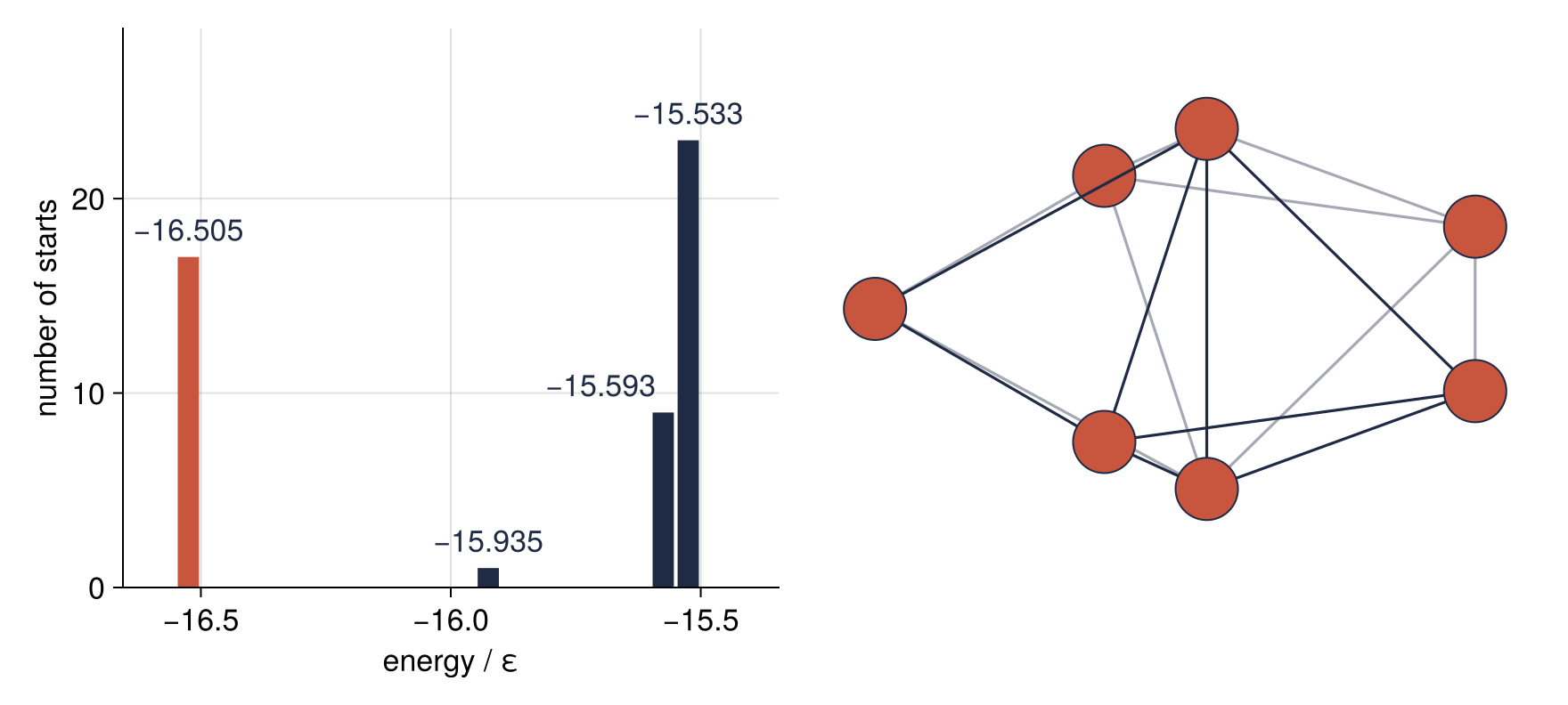
Left: how many of the fifty starts end at each energy, in ε. The red bar, 17 starts at −16.505 ε, is the global minimum; the tallest, 23 starts at −15.533 ε, is not. Right: the winning cluster, a ring of five atoms with one above and one below.

That is the picture from the opening. On the right the two tips sit top and bottom, the bond between them upright through the ring, and the faded lines are the bonds on the far side.

Pitfalls

Trusting the minimum without reading converged. In Step 4 Nelder-Mead reported −13.830 ε, believable for seven atoms and not a minimum: the trial points were there when the iteration budget ran out, which converged false admits. Read Optim.converged in every loop. If it is false, pass Optim.Options(iterations = 10_000) as the last argument of optimize, or switch to a gradient method and hand it the gradient. A true value promises only what Step 2 said, as the third pitfall shows.

A gradient that returns instead of filling. Compute the gradient as a new vector and assign it to G, and nothing happens:

function gradient_wrong!(G, x)
    G = ForwardDiff.gradient(energy, x)    # a new array; Optim's G is never written
    return G
end

w = optimize(energy, gradient_wrong!, x0, BFGS())
@printf("E = %.6f ε  converged = %s  iterations = %d  g_residual = %s\n",
        Optim.minimum(w), Optim.converged(w), Optim.iterations(w), Optim.g_residual(w))

E = -1.285777 ε  converged = false  iterations = 0  g_residual = NaN

Zero iterations, the energy of the start, and a gradient of NaN, the value Optim puts in its buffer before your function fills it. Inside the function G is a name bound to Optim's array: G = ... points the name at a new array, while G .= ... or G[i] = ... writes into the array the name points to. The same trap catches du in DifferentialEquations.jl from the ground up: the pendulum beyond small angles.

Starting atoms too close: the first step throws them apart. Lower d_min from 1.0 to 0.8 σ and run fifty starts again, with plain BFGS and with its first step capped:

rng = Xoshiro(1)                             # fresh seed: these starts do not depend on the cells above
starts = [random_start(7; d_min = 0.8) for _ in 1:50]
spread(r) = maximum(distances(Optim.minimizer(r)))       # largest pair distance at the end
for method in [BFGS(), BFGS(initial_stepnorm = 0.1)]
    runs = [optimize(energy, gradient!, s, method) for s in starts]
    E = Optim.minimum.(runs)
    @printf("initial_stepnorm = %-8s converged %2d of 50, above −15.5 ε %2d, spread over 5 σ %2d\n",
            method.initial_stepnorm, count(Optim.converged, runs), count(>(-15.5), E), count(r -> spread(r) > 5, runs))
    # + 0.0 turns the -0.0 of a rounded -1e-11 into 0.0
    method.initial_stepnorm === nothing && println("  energies: ", sort(unique(round.(E, digits = 3) .+ 0.0)))
end

initial_stepnorm = nothing  converged 50 of 50, above −15.5 ε 33, spread over 5 σ 33
  energies: [-16.505, -15.935, -15.593, -15.533, -9.104, -6.0, -3.0, -1.0, 0.0]
initial_stepnorm = 0.1      converged 50 of 50, above −15.5 ε  0, spread over 5 σ  0

Every run converged, and 33 of the plain ones are no seven-atom cluster: −9.104, −6, −3, and −1 ε are Step 3's bipyramid, a tetrahedron, a triangle, and a pair with the other atoms gone, and 0 ε is seven lone atoms. BFGS knows nothing of the curvature at the start, so its first step is the gradient itself. Two atoms 0.8 σ apart push on each other with a force of about 760 ε/σ, against 24 ε/σ at 1.0 σ. The line search, which picks the step length along that direction, accepts this step because the energy drops, and it sends atoms hundreds of σ away, where the attraction, \(24 r^{-7}\), is below g_abstol. Flat ground, test passed. Start no closer than about 1 σ, or cap the first step with initial_stepnorm, and run the neighbor count of Step 5 on the result.

Variations

Basin hopping by hand. Kick the best minimizer, Optim.minimizer(best) .+ 0.3 .* randn(rng, 21), minimize again, and keep the result if it is lower, in a loop. Wales and Doye gave the method its name in 1997, in the paper listed under further reading.
Thirteen atoms. Call random_start(13; side = 4.0): at side 2.5 practically no draw keeps thirteen atoms 1 σ apart, at 4.0 about one in sixty. Thirteen atoms have their lowest energy, −44.326801 ε, as an icosahedron. Tally how often fifty starts reach it and how many different energies they end at, and set that beside the seven-atom tally.
Bounds. optimize(energy, gradient!, lower, upper, x0, Fminbox(LBFGS())) keeps every coordinate between lower and upper, with -Inf or Inf for an open side. Atoms on a surface need \(z \ge 0\): a lower bound of 0 for every third coordinate.
Fitting. Least squares and maximum likelihood are minimizations too: the residual sum or the negative log-likelihood is the f you pass. For least squares LsqFit's curve_fit also returns the parameter errors, as in Fit a curve with error bars and draw a confidence band in Julia.

Cheat sheet

res = optimize(f, x0, BFGS())                     # x0 a flat vector; no method means NelderMead()
res = optimize(f, g!, x0, BFGS())                 # g!(G, x) fills G, never rebinds it
res = optimize(f, x0, BFGS(); autodiff = AutoForwardDiff())   # using ADTypes; f must accept any number type
LBFGS(), ConjugateGradient()                      # no full Hessian estimate, for many variables
optimize(f, g!, lower, upper, x0, Fminbox(LBFGS()))           # box constraints
Optim.minimizer(res), Optim.minimum(res)          # where it stopped and the value there
Optim.converged(res)                              # a stopping test passed, nothing more
Optim.f_calls(res), Optim.g_calls(res)            # cost meter; finite differences not in f_calls
optimize(f, g!, x0, BFGS(), Optim.Options(iterations = 10_000))
best = argmin(Optim.minimum, [optimize(f, g!, s, BFGS()) for s in starts])   # restarts