Numerical integration with QuadGK.jl: the area under a measured peak

The problem: how much light is in one spectral line?

Your spectrometer hands you 401 intensity readings in counts, one every 0.1 nm from 500 to 540 nm, with an emission line in the middle and a sloping background beneath it. The number you are after is the integral of the line alone, its area in counts·nm. It is proportional to the number of emitters: a concentration to a chemist, an oscillator strength to a physicist who knows that number. Any peak on a background asks for the same steps, be it a chromatogram, an X-ray diffraction pattern whose peak areas give the fractions of mineral phases, or a resonance in a vibration spectrum. Over all 401 readings the integral comes to 2856 counts·nm, and more than half of that is background.

There are two routes in Julia. Samples go through the trapezoid and Simpson rules, a few lines of plain Julia, since the language has no single standard function for them. A formula goes to quadgk from QuadGK.jl. It places its own sample points, hands back an estimate of its error next to the value, and accepts infinite limits as well as an integrand that goes to infinity at a known point. The formulas below are the line shape of this same peak and the period of the pendulum from DifferentialEquations.jl from the ground up: the pendulum beyond small angles, an integral whose integrand is infinite at one end.

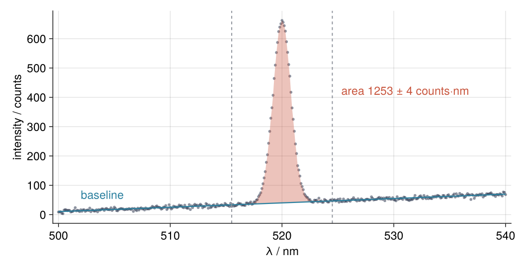
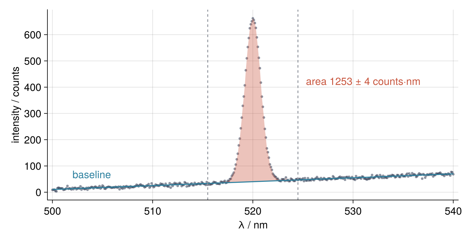
Simulated emission spectrum, counts against wavelength from 500 to 540 nm. Dots: measured points. Thin line: straight baseline fitted to the flanks. Shaded: the line area above the baseline between the dashed window edges, 1253 ± 4 counts·nm.

The shaded area is the answer, 1253 ± 4 counts·nm, and the simulation knows the truth, 1250. The uncertainty combines the noise and the baseline, and Step 6 draws the figure.

Setup

Install the packages once with import Pkg; Pkg.add(["QuadGK", "SpecialFunctions", "CairoMakie"]); LinearAlgebra, Statistics, Random, and Printf ship with Julia. The spectrum is simulated so that the truth is known. measure draws fresh noise on every call, and Step 6 calls it again to repeat the measurement.

using QuadGK: quadgk, quadgk_count
using SpecialFunctions: ellipk
using LinearAlgebra, Statistics, Random, Printf, CairoMakie

# the truth, which a real spectrometer never shows you
const AREA = 1250.0                 # line area, counts·nm
const CENTER, WIDTH = 520.0, 0.8    # nm: center and standard deviation of the line
const B0, B1 = 40.0, 1.5            # baseline: counts at the center, counts/nm
const NOISE = 4.0                   # standard deviation of the noise, counts

λ = range(500, 540, length = 401)   # wavelength, nm

function measure(rng)
    line = @. AREA / (WIDTH * sqrt(2π)) * exp(-0.5 * ((λ - CENTER) / WIDTH)^2)   # @. dots every operation
    return line .+ B0 .+ B1 .* (λ .- CENTER) .+ NOISE .* randn(rng, length(λ))
end

rng = Xoshiro(13)
counts = measure(rng)

const INK, ACCENT, SECOND, MUTED = "#1f2a44", "#c8553d", "#2a7f9e", "#8a8f98"
set_theme!(Theme(                   # the look of every figure below
    size = (770, 396), fontsize = 17,
    palette = (color = [INK, ACCENT, SECOND, MUTED],),
    Axis = (topspinevisible = false, rightspinevisible = false, xgridvisible = true, ygridvisible = true),
    Lines = (linewidth = 2.5,),
))

@printf("%d points, spacing %.1f nm, maximum %.0f counts\n", length(λ), step(λ), maximum(counts))

401 points, spacing 0.1 nm, maximum 662 counts

Step 1: Integrate sampled data with the trapezoid and Simpson rules

Look at the record first:

fig = Figure(size = (770, 352))
ax = Axis(fig[1, 1], xlabel = "λ / nm", ylabel = "intensity / counts", limits = ((499.5, 540.5), nothing))
scatter!(ax, λ, counts, color = INK, markersize = 6)
text!(ax, 528, 95, text = "background", color = MUTED)
fig

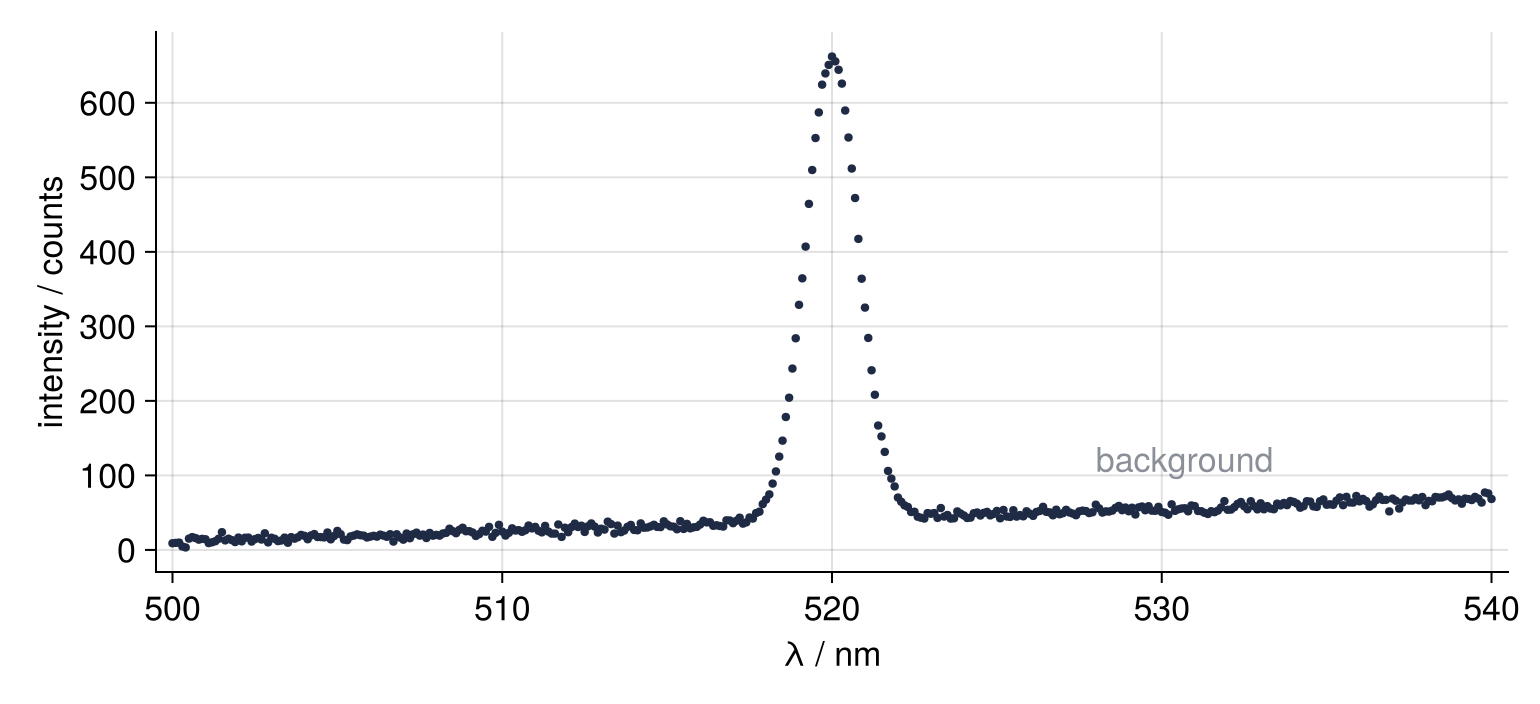
The simulated spectrum, intensity in counts against wavelength from 500 to 540 nm, one dot per reading. A narrow line near 520 nm peaks at 662 counts on a background that rises slowly from left to right.

The line stands near 520 nm, narrow against the 40 nm record, and reaches 662 counts with the background included. The background climbs toward long wavelengths, and the first and last 5 nm of the record hold nothing else.

The trapezoid rule connects neighboring readings by straight lines and sums the areas beneath them. Simpson's rule puts a parabola through every three neighbors instead, which needs an odd number of equally spaced points. With an even number, drop one end point, which on a spectrum like this holds only background, or use trapezoid:

trapezoid(x, y) = sum(diff(x) .* (y[1:end-1] .+ y[2:end])) / 2

function simpson(x, y)              # equally spaced x
    isodd(length(y)) || error("simpson needs an odd number of points")
    h = x[2] - x[1]
    return h / 3 * (y[1] + 4sum(y[2:2:end-1]) + 2sum(y[3:2:end-2]) + y[end])
end

@printf("trapezoid %8.2f counts·nm\n", trapezoid(λ, counts))
@printf("simpson   %8.2f counts·nm\n", simpson(λ, counts))

trapezoid  2855.75 counts·nm
simpson    2857.00 counts·nm

Trapezoid and Simpson differ by 0.04 %. The choice of rule is not what is wrong with 2856; the background inside it is.

Step 2: Find the peak, choose a window, subtract the baseline

Before the background can come off, you need to know where the line ends, and on a real record nobody tells you its position or its width. Read both from the data, in three moves.

First, a rough straight line fitted to the first and last 5 nm, which serves only to find the peak and its width; the baseline that counts comes once the window is known. A \ b with a tall matrix A, more rows than columns, returns the least-squares solution, so the two columns, ones and λ, fit a straight line. Second, the peak sits where the counts minus that line reach their maximum, and the full width at half maximum (FWHM) is how wide the line is at half its height, measured from the first to the last point that gets there. Third, the window reaches 2.5 FWHM to either side:

edge = (λ .< 505) .| (λ .> 535)
rough = [ones(count(edge)) λ[edge]] \ counts[edge]   # intercept and slope
net = counts .- (rough[1] .+ rough[2] .* λ)
peak = λ[argmax(net)]
above = λ[net .>= maximum(net) / 2]
fwhm = last(above) - first(above)
half = 2.5fwhm
@printf("peak at %.1f nm, FWHM %.1f nm, window ±%.1f nm\n", peak, fwhm, half)

peak at 520.0 nm, FWHM 1.8 nm, window ±4.5 nm

The width is good to a sample spacing or two, 0.1 to 0.2 nm, which is all a window needs. Step 3 checks that ±4.5 nm keeps the whole line.

With one line on a straight background, everything outside the window is flank, and the flanks get the real baseline. The design matrix X, one row per flank reading and one column per coefficient, counts wavelength from the peak, which makes the intercept equal to the background right under the line; Step 5 needs X again. Subtract the baseline and integrate the window alone:

win = abs.(λ .- peak) .<= half + 1e-9    # the slack keeps the edge points despite rounding
flank = .!win
X = [ones(count(flank)) λ[flank] .- peak]
p = X \ counts[flank]
intercept, slope = p
line = counts[win] .- (intercept .+ slope .* (λ[win] .- peak))
area = trapezoid(λ[win], line)

@printf("%d points in the window\n", count(win))
@printf("baseline under the peak %.2f counts, slope %.3f counts/nm\n", intercept, slope)
@printf("line area: trapezoid %.2f, simpson %.2f counts·nm\n", area, simpson(λ[win], line))

91 points in the window
baseline under the peak 40.08 counts, slope 1.487 counts/nm
line area: trapezoid 1252.65, simpson 1251.37 counts·nm

Now the area misses the true 1250 by under 3 counts·nm, and the two rules differ by 1.28 counts·nm. Whether 1.28 is large is a question for Step 5, which puts an uncertainty on the area, and for Pitfall 2.

Step 3: Integrate a formula with quadgk and read its error estimate

A formula can be evaluated anywhere, so quadgk(f, a, b) chooses the points itself. It cuts the interval into segments, denser where the function changes fast, and samples each segment at 15 interior points that form a Gauss-Kronrod rule, a weighted sum of function values at fixed positions; no sample lands on a segment's end.

Seven of the 15 points make a Gauss rule of their own, so every segment yields two answers for 15 evaluations, the Kronrod sum and the Gauss sum. Their difference is the segment's error estimate. quadgk adds up the estimates of all segments, splits the segment with the largest one, and repeats until the total is small enough. It returns two numbers, the value and that total.

The open question from Step 2 is whether the window holds the whole line. That is a ratio of two areas, so the height drops out. Use a unit-height Gaussian whose FWHM is the measured one; for a Gaussian the FWHM is 2.355 standard deviations. Put it at zero, for a reason Pitfall 1 shows. The total needs infinite limits:

σ = fwhm / (2sqrt(2log(2)))         # FWHM = 2.355 σ for a Gaussian
shape(u) = exp(-0.5 * (u / σ)^2)

total, err = quadgk(shape, -Inf, Inf)
@printf("total %.12f nm, error estimate %.1e\n", total, err)
@printf("exact %.12f nm\n", σ * sqrt(2π))

total 1.916040634976 nm, error estimate 9.3e-09
exact 1.916040634976 nm

All twelve digits match the exact σ√(2π). The fraction lost outside the window is the area of the two tails over the total, and each tail runs from the window edge to infinity:

for k in [1, 1.5, 2.5]
    tail, tail_err = quadgk(shape, k * fwhm, Inf)
    @printf("beyond ±%.1f FWHM: lost fraction %.1e, error estimate %.0e nm\n", k, 2tail / total, tail_err)
end

beyond ±1.0 FWHM: lost fraction 1.9e-02, error estimate 4e-11 nm
beyond ±1.5 FWHM: lost fraction 4.1e-04, error estimate 3e-13 nm
beyond ±2.5 FWHM: lost fraction 3.9e-09, error estimate 7e-18 nm

At ±1 FWHM the window would lose 1.9 % of the line, at ±1.5 FWHM 0.04 %, at ±2.5 FWHM 3.9e-9: Step 2's window keeps the whole Gaussian, and another line shape gets the same question (Variations). That last loss is smaller than 1.5e-8, the relative accuracy quadgk aims for by default. Computed as 1 − inside/total, the loss would be mostly error, while the tail itself comes with an estimate of 7e-18 nm. These estimates measure quadgk's arithmetic, not the noise in your data (Pitfall 2).

That accuracy is the keyword rtol, by default sqrt(eps()), and quadgk_count returns the number of evaluations as a third value:

for rtol in [sqrt(eps()), 1e-3]
    value, est, nevals = quadgk_count(shape, -half, half; rtol = rtol)
    @printf("rtol %.1e: %3d evaluations, value %.12f nm, error estimate %.1e\n", rtol, nevals, value, est)
end

rtol 1.5e-08: 135 evaluations, value 1.916040627443 nm, error estimate 1.8e-08
rtol 1.0e-03:  45 evaluations, value 1.916040627478 nm, error estimate 1.4e-04

At rtol = 1e-3 the work drops from 135 to 45 evaluations, and the value stays the same to ten digits while the estimate grows to 1.4e-4. The estimate is pessimistic, as usual, but no guarantee: Pitfall 1 shows an error estimate of zero for an integral of 1.9 nm.

Step 4: Handle singular points: the pendulum period

Energy conservation per unit mass gives the speed of a pendulum released from rest at \(\theta_0\):

\[\tfrac12 L^2\dot\theta^2 = gL(\cos\theta - \cos\theta_0) .\]

Solve for \(\dot\theta\), write \(dt = d\theta/\dot\theta\), and count four quarter swings, each from \(\theta_0\) down to 0, in one period:

\[T = 4\sqrt{\frac{L}{2g}}\int_0^{\theta_0}\frac{d\theta}{\sqrt{\cos\theta - \cos\theta_0}} .\]

At \(\theta_0\), where the bob stops, the integrand is infinite. Its area stays finite because the integrand grows only like \(1/\sqrt{\theta_0 - \theta}\) there, and quadgk copes because it never evaluates an end point. The exact answer is \(4\sqrt{L/g}\,K(m)\) with \(m = \sin^2(\theta_0/2)\) and \(K\) the complete elliptic integral of the first kind, which ellipk from SpecialFunctions evaluates with \(m\) as its argument:

g, L = 9.81, 1.0                    # m/s², m
θ0 = deg2rad(90)
integral, err, nevals = quadgk_count(θ -> 1 / sqrt(cos(θ) - cos(θ0)), 0, θ0)
T = 4 * sqrt(L / (2g)) * integral
T_exact = 4 * sqrt(L / g) * ellipk(sin(θ0 / 2)^2)
T0 = 2π / sqrt(g / L)                # small-angle period

@printf("T = %.6f s, small-angle T0 = %.3f s, T/T0 = %.4f, %d evaluations\n", T, T0, T / T0, nevals)
@printf("error estimate %.1e s, actual error %.1e s\n", 4 * sqrt(L / (2g)) * err, T - T_exact)

T = 2.367842 s, small-angle T0 = 2.006 s, T/T0 = 1.1803, 1305 evaluations
error estimate 3.1e-08 s, actual error -1.2e-08 s

This is the 2.367842 s that DifferentialEquations.jl found with a callback in the pendulum tutorial, now from one call instead of a solver run, and 18 % longer than the small-angle formula says. Here the error estimate is honest, within a factor of three of the actual error. It is not cheap: 1305 evaluations, almost ten times the 135 of the smooth window integral, because quadgk keeps halving the segment next to \(\theta_0\).

A singularity inside the interval is another matter. \(1/\sqrt{|x|}\) on \((-1, 1)\), a variant of an example on the QuadGK Examples page, integrates to exactly 4, and its infinity sits at 0, the middle of the interval:

f(x) = 1 / sqrt(abs(x))
try
    quadgk(f, -1, 1)
catch e
    showerror(stdout, e)
end
println()
value, est, nevals = quadgk_count(f, -1, 0, 1)
@printf("break point at 0: %.8f, error estimate %.1e, %d evaluations\n", value, est, nevals)

DomainError with 0.0:
integrand produced NaN in the interval (-1, 1)
break point at 0: 3.99999996, error estimate 5.7e-08, 2580 evaluations

The middle of a segment is a node of both the Gauss and the Kronrod rule. There 1/0 is Inf, so both sums are Inf, their difference is Inf - Inf, which is NaN, and quadgk throws an error rather than return a number it cannot judge. Extra arguments between the limits are break points: quadgk(f, -1, 0, 1) integrates over (−1, 0) and (0, 1), the singularity sits at an end of both, where no rule evaluates, and the answer is good to eight digits, the default tolerance.

Step 5: Put an uncertainty on the peak area

The uncertainty of a weighted sum follows from its weights, and the trapezoid area is one: \(A = \sum_i w_i y_i\), with weights fixed by the wavelengths. To see them, feed trapezoid a spectrum that is zero everywhere except for a 1 at point \(i\); what comes out is \(w_i\):

n = count(win)
w = [trapezoid(λ[win], (1:n) .== i) for i in 1:n]
println("weights / nm: ", round.(w[1:3], digits = 3), " ... ", round.(w[end-1:end], digits = 3))

weights / nm: [0.05, 0.1, 0.1] ... [0.1, 0.05]

Every inner point weighs 0.1 nm, the two end points half that. Two sources make \(A\) uncertain. The first is the noise, whose standard deviation \(\sigma_y\) is read off the flanks: the scatter of their 310 readings around the fitted baseline, with 310 − 2 in the denominator, length(r) - 2 in the code, because the fit used up two parameters. For independent readings the variance of a weighted sum is \(\sigma_y^2\sum_i w_i^2\).

The second is the baseline. Under the window it contributes \(g_1a + g_2b\): the intercept \(a\) and the slope \(b\), weighted by \(g_1 = \sum_i w_i\) and \(g_2 = \sum_i w_i(\lambda_i - \lambda_\text{peak})\), which form the vector \(\mathbf g\). Both coefficients come from the same flank readings, so their errors are correlated, and their covariance matrix \(C\) records it: the variances of \(a\) and \(b\) on its diagonal, how the two move together off it. The variance of the sum is \(g_1^2\operatorname{var}a + 2g_1g_2\operatorname{cov}(a, b) + g_2^2\operatorname{var}b\), which is \(\mathbf g^\mathsf{T} C\,\mathbf g\) written out. For a least-squares fit whose readings share one independent noise level, \(C\) is σy^2 * inv(X' * X), with X' the transpose of X. vcov from LsqFit.jl returns the same matrix for a fit without weights, and Fit a curve with error bars and draw a confidence band in Julia uses it on a weighted fit:

r = counts[flank] .- X * p                  # flank residuals
σy = sqrt(sum(r .^ 2) / (length(r) - 2))
noise = σy * sqrt(sum(w .^ 2))

C = σy^2 * inv(X' * X)
g = [sum(w), sum(w .* (λ[win] .- peak))]
base = sqrt(g' * C * g)
dA = hypot(noise, base)                     # √(noise² + base²)

@printf("σy %.2f counts -> noise term %.2f counts·nm\n", σy, noise)
@printf("g = (%.1f nm, %.1f nm²), intercept ± %.3f counts -> baseline term %.2f counts·nm\n",
        g[1], g[2], sqrt(C[1, 1]), base)
@printf("A = %.1f ± %.1f counts·nm\n", area, dA)
w_simpson = [simpson(λ[win], (1:n) .== i) for i in 1:n]
@printf("noise term with Simpson weights %.2f counts·nm\n", σy * sqrt(sum(w_simpson .^ 2)))

σy 4.00 counts -> noise term 3.79 counts·nm
g = (9.0 nm, 0.0 nm²), intercept ± 0.227 counts -> baseline term 2.05 counts·nm
A = 1252.7 ± 4.3 counts·nm
noise term with Simpson weights 4.00 counts·nm

\(\sigma_y\) comes out at 4.00 counts, against the true 4. Reading it off the flanks assumes the same noise under the peak, true here and false for counting data (Variations). \(\mathbf g\) is (9.0 nm, 0): the window is symmetric about the wavelength the baseline is measured from, so the slope drops out and the baseline term is 9.0 nm × 0.227 counts. Window and flanks share no readings, so the two terms are independent and add in squares: \(A\) = 1252.7 ± 4.3 counts·nm, 0.6 standard deviations from the true 1250. The Simpson line is for Pitfall 2.

Step 6: Check the uncertainty by repeating the measurement

A simulation can do what a real measurement cannot: measure again. Each of 2000 reruns draws fresh noise with measure, fits its own baseline to the flanks with the same X, since the window stays fixed, and integrates the window. The do block is the function that map applies to each element of 1:2000:

areas = map(1:2000) do _
    y = measure(rng)
    q = X \ y[flank]                        # this rerun's intercept and slope
    trapezoid(λ[win], y[win] .- (q[1] .+ q[2] .* (λ[win] .- peak)))
end
@printf("2000 reruns: mean %.2f, standard deviation %.2f counts·nm\n", mean(areas), std(areas))

2000 reruns: mean 1249.91, standard deviation 4.39 counts·nm

The areas scatter by 4.39 counts·nm around 1249.91. The propagated 4.3 is right to 2 %, and the method has no bias that 2000 reruns can see. Here is the figure from the top, drawn from these variables:

baseline = intercept .+ slope .* (λ .- peak)
fig = Figure()
ax = Axis(fig[1, 1], xlabel = "λ / nm", ylabel = "intensity / counts", limits = ((499.5, 540.5), nothing))
scatter!(ax, λ, counts, color = (INK, 0.5), markersize = 6)
band!(ax, λ[win], baseline[win], counts[win], color = (ACCENT, 0.35))
lines!(ax, λ, baseline, color = SECOND, linewidth = 1.7)    # drawn over the dots
vlines!(ax, [peak - half, peak + half], color = MUTED, linestyle = :dash, linewidth = 1.4)
text!(ax, 502, 45, text = "baseline", color = SECOND)
text!(ax, peak + half + 0.8, 400, text = @sprintf("area %.0f ± %.0f counts·nm", area, dA), color = ACCENT)
fig

Intensity in counts against wavelength in nm. Dots: the measured spectrum. Blue line: the straight baseline fitted to the flanks. Red fill: the line area above it between the dashed window edges, 1253 ± 4 counts·nm.

Pitfalls

quadgk returns zero for a peak it never saw. Shift the Step 3 shape to the real line at 520 nm and give quadgk infinite limits, or 0 and 2000 nm:

for (a, b) in [(-Inf, Inf), (0, 2000), (peak - 8, peak + 8)]
    value, est, nevals = quadgk_count(x -> shape(x - peak), a, b)
    @printf("from %6.1f to %6.1f nm: %.5f nm, error estimate %.0e, %3d evaluations\n", a, b, value, est, nevals)
end

from   -Inf to    Inf nm: 0.00000 nm, error estimate 0e+00,  15 evaluations
from    0.0 to 2000.0 nm: 0.00000 nm, error estimate 0e+00,  15 evaluations
from  512.0 to  528.0 nm: 1.91604 nm, error estimate 2e-09, 165 evaluations

The first two lines report zero, with an error estimate of zero, after one segment of 15 evaluations. On (−Inf, Inf) quadgk substitutes \(x = t/(1 - t^2)\) to make the interval finite, so its first samples crowd around \(x = 0\), far from 520 nm; on (0, 2000) they spread over 2000 nm. Either way all 15 miss the 2 nm the line occupies, the Kronrod and Gauss sums are both zero, so is their difference, and an estimate of zero meets any tolerance. The fix is limits that hug the peak, as in the third line, or a shift that puts the peak at zero before infinite limits. When quadgk reports an estimate of exactly zero for an integral that cannot be zero, it has not seen your function.

Reporting an integration error as the uncertainty. Someone reports 1252.7 ± 1.3 counts·nm, with the 1.3 taken from the gap between trapezoid and Simpson in Step 2, or quotes the far smaller error estimate of quadgk run on an interpolation, a function that joins the samples so that quadgk can evaluate it between them. Either understates Step 5's 4.3 by more than a factor of three. Each tells you how faithfully a rule sums the readings you happen to have; neither knows that a second measurement would give different readings. An interpolation goes through every noisy reading, so a precise integral of it is a precise integral of the noise. Report the propagated uncertainty and set the rule difference against it. Nor does a higher-order rule shrink the uncertainty. Simpson's weights alternate between 4/3 and 2/3 of the spacing where the trapezoid gives every inner point the spacing itself, and for the same total, unequal weights have a larger \(\sum_i w_i^2\), so the noise term rises from 3.79 to 4.00 counts·nm.

Summing instead of integrating. Julia has no trapz in Base, so sum(counts) is the shortcut people reach for:

@printf("%.1f\n", sum(counts))

28596.1

Ten times the 2856 of Step 1. A sum is in counts·sample, because the spacing of 0.1 nm is missing; integrate with the spacing, as trapezoid(x, y) does. An integral carries the unit of \(y\) times the unit of \(x\), here counts·nm. Plot the same line against wavenumber or photon energy and its area changes, number and unit both.

Variations

A running integral. [0; cumsum(diff(x) .* (y[1:end-1] .+ y[2:end]) ./ 2)] is the area from the first point up to each point: the energy a power log adds up to, or the wavelength that splits a line's area in half. NumericalIntegration.jl, from JuliaMath, packages this as cumul_integrate(x, y), next to integrate(x, y) for the whole area.
A Lorentzian or pseudo-Voigt line. Diffraction peaks and many spectral lines are closer to a pseudo-Voigt, a weighted sum of a Gaussian and a Lorentzian, and Lorentzian wings reach past any window: on a Lorentzian shape the Step 3 check finds only \((2/\pi)\arctan 5\), 87 %, inside ±2.5 FWHM. Fit the line shape as in the Julia fit recipe and hand the fitted model, shifted to zero, to quadgk with infinite limits. With many peaks, cut the record into stretches that each hold one peak and flanks free of any neighbor's tail: argmax finds only one peak, and a tail in the flanks lifts the baseline.
Counting data. Photon and X-ray counts have a variance equal to their expected count, so the noise is larger under the peak than on the flanks. For raw detector counts, not rescaled or background-subtracted by instrument software, two things change. The noise term becomes sqrt(sum(w .^ 2 .* counts[win])), the counts, background included, serving as variances. The baseline fit weights each flank reading by 1/countsᵢ: divide its row of X and its count by √countsᵢ, fit as before, and C = inv(Xw' * Xw), with Xw the scaled X and no σy. These fit weights, unrelated to the integration weights w, are what the fit recipe passes as PrecisionWeights(1 ./ sigma .^ 2), with σᵢ² = countsᵢ.
A Fourier-type integral. quadgk takes complex-valued integrands as they are: quadgk(x -> shape(x) * cis(-2π * ν * x), -Inf, Inf), with cis(φ) = \(e^{i\varphi}\), is the Fourier transform of the line shape at ν in 1/nm and reproduces the exact \(\sigma\sqrt{2\pi}\,e^{-2\pi^2\sigma^2\nu^2}\). What it means is the subject of The Fourier transform in Julia: asking a signal how much of each frequency it contains.

Cheat sheet

trapezoid(x, y) = sum(diff(x) .* (y[1:end-1] .+ y[2:end])) / 2   # always with x; unit(y) × unit(x)
simpson(x, y)                                       # odd number of equally spaced points; even: drop an end point
above = x[net .>= maximum(net) / 2]; fwhm = last(above) - first(above)   # net: y minus a rough baseline; ±2.5 FWHM for a Gaussian
X = [ones(count(flank)) x[flank] .- peak]; p = X \ y[flank]   # baseline from the flanks only
I, E = quadgk(f, a, b)                              # E is Kronrod minus Gauss: numerical, not your uncertainty
quadgk(f, -Inf, Inf); quadgk(f, a, c, b)            # center a peak at zero first; c: break point at a singularity
I, E, nevals = quadgk_count(f, a, b; rtol = 1e-8)   # default rtol ≈ 1.5e-8; loosen only for expensive f
w = [trapezoid(x[win], (1:n) .== i) for i in 1:n]   # n = count(win); the area is sum(w .* y[win])
C = σy^2 * inv(X' * X); g = [sum(w), sum(w .* (x[win] .- peak))]   # X' is the transpose
dA = hypot(σy * sqrt(sum(w .^ 2)), sqrt(g' * C * g))   # noise and baseline add in squares