The angular spectrum method with numpy.fft: a laser beam and a slit

The problem: how far does a laser beam stay parallel, and what does a slit do to light?

A helium-neon laser emits red light at λ = 633 nm. Take a beam of radius \(w_0 = 1\) mm at its waist. It looks parallel, and it is not. Over the Rayleigh range \(z_R = \pi w_0^2/\lambda\), 4.96 m here, the area of its cross-section doubles, and at 10 m the radius is 2.249 mm. The angular spectrum method computes that spreading from the field at the start alone, with two fast Fourier transforms.

The second case is a plane wave through a slit 0.5 mm wide. Right behind it is the slit's shadow, with ripples at its edges; far away is the sinc² pattern of the textbook. The Fresnel number \(N_F = a^2/(\lambda z)\) decides which, with \(a\) the half-width of the slit: it compares \(a\) with \(\sqrt{\lambda z}\), the width over which a wave smears out on its way over a distance \(z\). Well above 1 you see the shadow, well below 1 the sinc², and for this slit \(N_F = 1\) at 9.9 cm.

Each Cartesian component of the electric field obeys the same wave equation, and for a beam and a slit much wider than the wavelength the polarization does not mix in, so one complex number per point describes the light. The method takes that field apart into plane waves with a Fourier transform, moves each by multiplying it with a phase, and adds them back up.

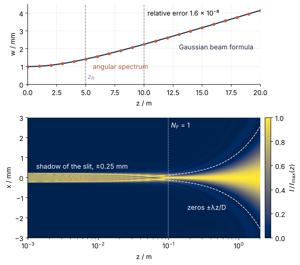
Top: laser beam radius in mm against distance up to 20 m, simulation dots on the Gaussian beam formula, error 1.6e-8 at 10 m. Bottom: intensity behind a 0.5 mm slit, position across the slit against distance on a log scale; the sharp shadow widens into the sinc² pattern past the Fresnel number 1 line at 10 cm.

At the top, the simulated beam radius sits on the formula out to 20 m, 1.6 × 10⁻⁸ off at 10 m, and that difference is the formula's fault, as Step 3 shows. At the bottom is the light behind the slit, each distance scaled to its own maximum: the shadow turns into the sinc² past the line \(N_F = 1\). Step 6 draws the figure.

Setup

import warnings

import numpy as np
import matplotlib.pyplot as plt

wavelength = 633e-9                 # m, helium-neon laser
k = 2 * np.pi / wavelength          # 1/m
w0 = 1e-3                           # m, beam radius at the waist
slit = 0.5e-3                       # m, slit width D
a = slit / 2                        # m, half-width, the length in the Fresnel number

plt.rcParams.update({
    "figure.figsize": (7, 3.6), "figure.dpi": 110,
    "axes.spines.top": False, "axes.spines.right": False,
    "axes.grid": True, "grid.alpha": 0.25,
    "font.size": 11, "lines.linewidth": 1.8,
})
INK, ACCENT, SECOND, MUTED = "#1f2a44", "#c8553d", "#2a7f9e", "#8a8f98"

z_R = np.pi * w0**2 / wavelength
print(f"Rayleigh range z_R = {z_R:.2f} m, N_F = 1 behind the slit at z = {a**2 / wavelength:.3f} m")

Rayleigh range z_R = 4.96 m, N_F = 1 behind the slit at z = 0.099 m

Step 1: Sample the laser beam on a grid

At its waist the beam has the amplitude \(E_0 = \exp(-r^2/w_0^2)\), a Gaussian whose intensity \(|E_0|^2\) falls to \(1/e^2\) at \(r = w_0\). Sample it on 512 × 512 points 0.2 mm apart, centered on the beam. The radius is measured from the intensity itself: \(\exp(-2x^2/w^2)\) is a Gaussian with standard deviation \(w/2\), so twice the standard deviation of the intensity across \(x\) is \(w\), and unlike a fit it stays defined when the beam is no longer Gaussian.

N, dx = 512, 0.2e-3
x = (np.arange(N) - N // 2) * dx
X, Y = np.meshgrid(x, x)
E0 = np.exp(-(X**2 + Y**2) / w0**2)

def beam_radius(E, X):
    """1/e² radius of a centered beam: twice the standard deviation of the intensity in x."""
    I = np.abs(E) ** 2
    return 2 * np.sqrt(np.sum(I * X**2) / np.sum(I))

print(f"{w0 / dx:.0f} points per waist, window {N * dx * 1e3:.1f} mm = {N * dx / w0:.0f} waists")
print(f"spectrum at the highest wavenumber pi/dx: {np.exp(-(np.pi / dx * w0) ** 2 / 4):.1e} of its peak")
print(f"beam radius at z = 0: {beam_radius(E0, X) * 1e3:.5f} mm")

5 points per waist, window 102.4 mm = 102 waists
spectrum at the highest wavenumber pi/dx: 1.6e-27 of its peak
beam radius at z = 0: 1.00000 mm

Five points per waist look sparse, and they are enough. The grid holds wavenumbers up to \(\pi/\Delta x\), the Nyquist limit of the prerequisite, and the field must have nothing beyond it. A Gaussian's spectrum falls as \(\exp(-k^2 w_0^2/4)\), which at five points per waist leaves 10⁻²⁷ at the limit, far below rounding. The rule of thumb: about five points across the finest feature of the field. The window, 102 waists wide, is sized for the beam at 20 m, not at the start; Step 4 says how.

Step 2: Split the field into plane waves and move each one

Light of one frequency is a field \(E(\mathbf r)\,e^{-i\omega t}\), and for it the wave equation reduces to the Helmholtz equation, \(\nabla^2 E + k^2 E = 0\) with \(k = 2\pi/\lambda\). A plane wave \(\exp(i(k_x x + k_y y + k_z z))\) solves it when \(k_x^2 + k_y^2 + k_z^2 = k^2\). So \(k_x\) and \(k_y\) fix \(k_z\), and moving the wave by \(z\) multiplies it by \(\exp(ik_z z)\). Split the field into plane waves, move each, add them up:

\[E(x, y, z) = \mathcal F^{-1}\Big[\mathcal F[E_0]\;\exp\big(iz\sqrt{k^2 - k_x^2 - k_y^2}\,\big)\Big].\]

With the time dependence \(e^{-i\omega t}\), the wave \(\exp(i(k_x x + k_z z))\) with \(k_z > 0\) travels toward \(+z\). NumPy's inverse transform builds the field from terms \(\exp(+ik_x x)\), so multiplying each by \(\exp(+ik_z z)\) moves it forward. np.fft.fft2 is the transform of the prerequisite applied along each axis in turn. np.fft.fftfreq lists the frequencies in cycles per meter, which \(2\pi\) turns into wavenumbers, in the order fft2 stores them, so no fftshift is needed (the MRI tutorial explains the order):

print("fftfreq order:", np.fft.fftfreq(8, d=1 / 8))

def propagate(E, dx, z):
    """Angular spectrum propagation of a square field E, sampled at spacing dx, over a distance z."""
    kx = 2 * np.pi * np.fft.fftfreq(E.shape[0], d=dx)       # wavenumbers in NumPy's order
    KX, KY = np.meshgrid(kx, kx)
    kz = np.sqrt((k**2 - KX**2 - KY**2).astype(complex))     # imaginary for evanescent waves
    return np.fft.ifft2(np.fft.fft2(E) * np.exp(1j * kz * z))

fftfreq order: [ 0.  1.  2.  3. -4. -3. -2. -1.]

Where \(k_x^2 + k_y^2 > k^2\) the root is imaginary, and the complex square root turns the phase factor into a decay \(\exp(-|k_z| z)\), over a fraction of a wavelength once \(k_\perp\) is well above \(k\). These evanescent waves appear on a grid only below \(\Delta x = \lambda/\sqrt 2\), first in its corners, where \(k_\perp = \sqrt 2\,\pi/\Delta x\). At 0.2 mm this grid has none; the third pitfall shows what goes wrong with them. The discrete method is exact for a field that is periodic and band-limited on the grid. Two checks:

power = lambda E: np.sum(np.abs(E) ** 2)
E10 = propagate(E0, dx, 10.0)
print(f"largest |E(z = 0) - E0|:    {np.max(np.abs(propagate(E0, dx, 0.0) - E0)):.1e}")
print(f"power at 10 m / power at 0: {power(E10) / power(E0):.15f}")

largest |E(z = 0) - E0|:    2.5e-16
power at 10 m / power at 0: 1.000000000000000

Zero distance gives back the field to rounding, and the power after 10 m equals the power at the start to 15 digits, because \(|\exp(ik_z z)| = 1\) for every propagating wave.

Step 3: Check the beam radius against the Gaussian beam formula

For a wave at a small angle to the axis, \(k_\perp^2 = k_x^2 + k_y^2\) is small compared with \(k^2\), and \(k_z = \sqrt{k^2 - k_\perp^2} \approx k - k_\perp^2/(2k)\). That is the paraxial approximation. The paraxial wave equation, whose plane waves have this \(k_z\), has the Gaussian beam as an exact solution, with the radius \(w(z) = w_0\sqrt{1 + (z/z_R)^2}\); Saleh and Teich derive it (Further reading). Propagate to 41 distances from 0 to 20 m and compare:

z_beam = np.linspace(0, 20, 41)
w_sim = np.array([beam_radius(propagate(E0, dx, z), X) for z in z_beam])
w_formula = w0 * np.sqrt(1 + (z_beam / z_R) ** 2)
for z, ws, wf in zip(z_beam[::10], w_sim[::10], w_formula[::10]):
    print(f"z = {z:4.1f} m   simulated {ws * 1e3:.5f} mm   formula {wf * 1e3:.5f} mm")

i10 = 20                                                     # z_beam[20] = 10 m
print(f"relative error at 10 m: {w_sim[i10] / w_formula[i10] - 1:.4e}")

xf = (np.arange(2 * N) - N) * dx / 2                         # twice the points, half the spacing
Xf, Yf = np.meshgrid(xf, xf)
Ef = propagate(np.exp(-(Xf**2 + Yf**2) / w0**2), dx / 2, 10.0)
print(f"the same on the finer grid: {beam_radius(Ef, Xf) / w_formula[i10] - 1:.4e}")

z =  0.0 m   simulated 1.00000 mm   formula 1.00000 mm
z =  5.0 m   simulated 1.41949 mm   formula 1.41949 mm
z = 10.0 m   simulated 2.24941 mm   formula 2.24941 mm
z = 15.0 m   simulated 3.18349 mm   formula 3.18349 mm
z = 20.0 m   simulated 4.15203 mm   formula 4.15203 mm
relative error at 10 m: 1.6271e-08
the same on the finer grid: 1.6271e-08

Five digits of agreement at every distance, and a relative error of 1.6 × 10⁻⁸ at 10 m. An error this small is easy to take for rounding, but it grows with \(z\) and does not move on a grid with four times as many points. It belongs to the formula: the formula uses the paraxial \(k_z\), the propagator the exact one, which makes the beam spread slightly faster, by

\[\frac{\Delta w}{w} = \frac{\theta^2}{2}\,\frac{(z/z_R)^2}{1 + (z/z_R)^2},\]

with \(\theta = \lambda/(\pi w_0)\) the divergence angle of the beam. Put the paraxial \(k_z\) into the propagator, and the difference should vanish:

theta = wavelength / (np.pi * w0)                            # rad
u = (10.0 / z_R) ** 2
print(f"divergence angle {theta * 1e3:.3f} mrad, predicted correction at 10 m: {theta**2 / 2 * u / (1 + u):.4e}")

kx = 2 * np.pi * np.fft.fftfreq(N, d=dx)
KX, KY = np.meshgrid(kx, kx)
kz_paraxial = k - (KX**2 + KY**2) / (2 * k)
E_paraxial = np.fft.ifft2(np.fft.fft2(E0) * np.exp(1j * kz_paraxial * 10.0))
print(f"paraxial propagator against the formula at 10 m: {beam_radius(E_paraxial, X) / w_formula[i10] - 1:.1e}")

divergence angle 0.201 mrad, predicted correction at 10 m: 1.6287e-08
paraxial propagator against the formula at 10 m: 7.4e-11

Measured 1.6271 × 10⁻⁸, predicted 1.6287 × 10⁻⁸. The last digits are lost to rounding: the phase \(k_z z\) is 10⁸ rad at 10 m, and a double stores it to about 10⁻⁸ rad. With the paraxial \(k_z\) the simulation matches the formula to 7 × 10⁻¹¹. The method is more accurate than the formula you were checking it against.

Step 4: Choose the grid for the slit: resolution and window

The slit is long in \(y\), so the field is one-dimensional, and the propagator is Step 2's with fft in place of fft2:

def propagate_1d(E, dx, z):
    kx = 2 * np.pi * np.fft.fftfreq(E.size, d=dx)
    kz = np.sqrt((k**2 - kx**2).astype(complex))
    return np.fft.ifft(np.fft.fft(E) * np.exp(1j * kz * z))

Resolution. Step 1's rule: five points across the finest feature. Behind a slit the finest feature is the edge ripple, about \(\sqrt{\lambda z}\) wide and narrowest close to the slit. Step 6's map starts at 1 mm, where the ripple is 25 µm, so Δx = 5 µm, 100 points across the slit. A top-hat's spectrum never falls to zero, so this is a compromise, and Step 5's comparison with sinc² checks it.

Window. The transfer function \(\exp(ik_z z)\) is sampled in \(k_x\) at spacing \(2\pi/L\), with \(L = N\Delta x\) the window, and it does not alias as long as its phase changes by less than π between neighbors: \(z\,(k_x/k_z)\,(2\pi/L) < \pi\). The product \(zk_x/k_z\) is how far that plane wave moves sideways, so the condition says that the steepest wave on the grid moves less than half a window. At \(k_x = \pi/\Delta x\), with \(k_z \approx k\), it becomes \(z \le N\Delta x^2/\lambda\).

The slit gets \(2^{16}\) points, a window of 33 cm and \(z_{\max}\) of 2.6 m. The test: propagate to 2 m on smaller windows, \(2^{13}\) and \(2^{14}\) points, whose \(z_{\max}\) falls short, and compare with this reference:

def z_max(N, dx):
    """Largest distance before the transfer function aliases."""
    return N * dx**2 / wavelength

def slit_field(N, dx):
    x = (np.arange(N) - N / 2 + 0.5) * dx        # half-sample offset: exactly 100 samples inside |x| < a
    return x, (np.abs(x) < a).astype(complex)

def near_axis(p):
    """Intensity at 2 m on a grid of 2^p points, at the same 2000 positions |x| < 5 mm on every grid."""
    x_p, E_p = slit_field(2**p, dx_slit)
    return np.abs(propagate_1d(E_p, dx_slit, 2.0)[np.abs(x_p) < 5e-3]) ** 2

dx_slit = 5e-6
print(f"edge ripple at z = 1 mm: {np.sqrt(wavelength * 1e-3) * 1e6:.0f} µm = {np.sqrt(wavelength * 1e-3) / dx_slit:.0f} points")
I_ref = near_axis(16)
print(f"reference N = 2^16: window {2**16 * dx_slit * 1e3:4.0f} mm, z_max = {z_max(2**16, dx_slit):4.2f} m")
for p in [13, 14]:
    diff = np.max(np.abs(near_axis(p) - I_ref)) / I_ref.max()
    print(f"          N = 2^{p}: window {2**p * dx_slit * 1e3:4.0f} mm, z_max = {z_max(2**p, dx_slit):4.2f} m, "
          f"intensity at 2 m off by {diff * 100:4.1f} %")

w20 = w0 * np.sqrt(1 + (20 / z_R) ** 2)
print(f"beam grid of Step 1: z_max = {z_max(N, dx):.0f} m; at 20 m the radius is {w20 * 1e3:.2f} mm, "
      f"the intensity 1e-16 of its peak at ±{w20 * np.sqrt(np.log(1e16) / 2) * 1e3:.1f} mm, the window ±{N * dx / 2 * 1e3:.1f} mm")

edge ripple at z = 1 mm: 25 µm = 5 points
reference N = 2^16: window  328 mm, z_max = 2.59 m
          N = 2^13: window   41 mm, z_max = 0.32 m, intensity at 2 m off by  6.6 %
          N = 2^14: window   82 mm, z_max = 0.65 m, intensity at 2 m off by  2.1 %
beam grid of Step 1: z_max = 32 m; at 20 m the radius is 4.15 mm, the intensity 1e-16 of its peak at ±17.8 mm, the window ±51.2 mm

For the slit at 2 m the error grows as \(z_{\max}\) falls below it: 2.1 % at 0.65 m, 6.6 % at 0.32 m. The condition is a worst case, light at the highest wavenumber on the grid, which a sharp edge has. A smooth field spreads only as fast as its own steepest wave, and the window just has to hold it at the largest \(z\): the beam needs ±17.8 mm at 20 m and has ±51.2 mm, enough even for the worst case up to 32 m. For your own field: with sharp edges, size the window by \(z \le N\Delta x^2/\lambda\); when it is smooth, by its width at the largest \(z\); either way, double \(N\) once and check that the answer does not move.

Step 5: Find the far field with the Fresnel number

Propagate the slit to the three distances where \(N_F\) is 10, 1, and 0.1: 9.9 mm, 9.9 cm, and 99 cm. Far away, in the Fraunhofer limit, the pattern is the slit's Fourier transform with the spatial frequency read as \(x/(\lambda z)\). That is \(\mathrm{sinc}^2(Dx/(\lambda z))\), with \(D = 2a\) the slit width and first zeros at \(x = \pm\lambda z/D\), and its height on the axis is \(D^2/(\lambda z)\) for an incident intensity of 1:

x_s, E_slit = slit_field(2**16, dx_slit)
view = np.abs(x_s) < 4e-3                                    # where the sinc² is compared
fig, axes = plt.subplots(3, 1, figsize=(7, 6.6))
for ax, N_F, half in zip(axes, [10, 1, 0.1], [0.5, 1.0, 4.0]):
    z = a**2 / (wavelength * N_F)
    I = np.abs(propagate_1d(E_slit, dx_slit, z)) ** 2
    sinc2 = np.sinc(slit * x_s / (wavelength * z)) ** 2
    deviation = np.max(np.abs(I[view] / I[view].max() - sinc2[view]))
    print(f"N_F = {N_F:4}  z = {z * 100:5.2f} cm  on axis {I[np.argmin(np.abs(x_s))]:6.3f}, "
          f"Fraunhofer {slit**2 / (wavelength * z):6.3f}, max |I/I_max - sinc²| = {deviation * 100:5.1f} %, peak {I.max():.2f}")
    if N_F < 1:                                              # far field: sinc² as the line, simulation as dots
        ax.plot(x_s * 1e3, I.max() * sinc2, color=INK)
        ax.plot(x_s[view][::40] * 1e3, I[view][::40], "o", color=ACCENT, ms=4)
        ax.text(0.7, 0.3, "sinc²", color=INK)
        ax.text(1.6, 0.05, "simulation", color=ACCENT)
    else:
        ax.plot(x_s * 1e3, I, color=ACCENT)
    for edge in [-a, a]:
        ax.axvline(edge * 1e3, color=MUTED, lw=1, ls="--")
    if N_F == 10:
        ax.text(0.27, 1.15, "slit edge", color=MUTED)
    ax.text(0.02, 0.85, f"$N_F$ = {N_F}, z = {z * 100:.2g} cm", transform=ax.transAxes)
    ax.set(xlim=(-half, half), xlabel="x / mm", ylabel="I / I₀")
fig.tight_layout()
plt.show()

N_F =   10  z =  0.99 cm  on axis  0.882, Fraunhofer 40.000, max |I/I_max - sinc²| = 100.0 %, peak 1.42
N_F =    1  z =  9.87 cm  on axis  1.578, Fraunhofer  4.000, max |I/I_max - sinc²| =  60.6 %, peak 1.58
N_F =  0.1  z = 98.74 cm  on axis  0.397, Fraunhofer  0.400, max |I/I_max - sinc²| =   0.4 %, peak 0.40

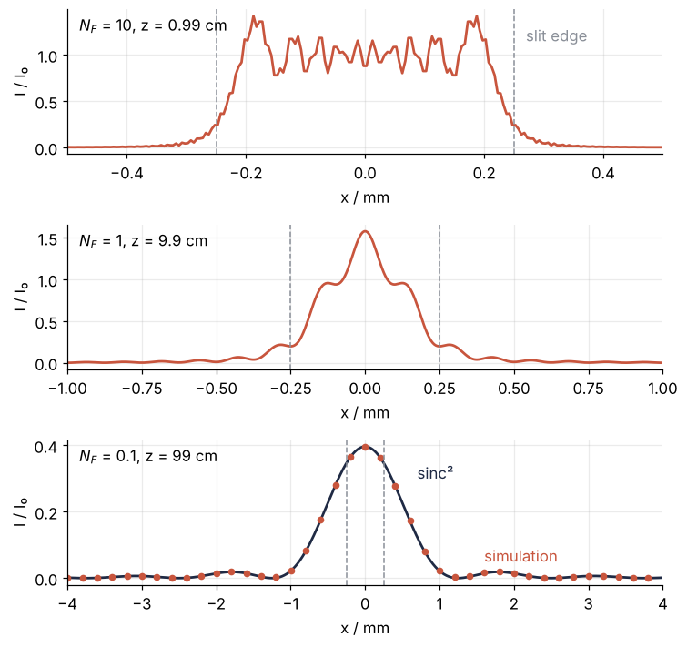
Intensity behind a 0.5 mm slit against position x in mm, at Fresnel numbers 10, 1, and 0.1. At 10 the shadow with edge ripples, at 1 a central peak with shoulders, at 0.1 the simulation lies on the sinc² curve.

At \(N_F = 10\) the light is still the shadow of the slit, with edge ripples that overshoot to 1.42, and the Fraunhofer formula is off by a factor of 45 on the axis. At \(N_F = 1\) the shadow has gone and the profile is still 61 % away from the sinc². At \(N_F = 0.1\) the profile is the sinc² to 0.4 %, and the height on the axis is right to 1 %. That is the test for "far" in any setup: compute \(N_F\) with the half-width of the aperture, and once it is well below 1 the Fourier transform of the aperture is the answer.

Step 6: Draw the beam radius and the slit map

The map needs the intensity at 240 distances from 1 mm to 2 m, spaced evenly on a log scale. The slit's spectrum does not depend on \(z\), so it is computed once and only the phase factor changes from row to row. Each row is divided by its maximum, so that the far field stays visible as it dims:

z_map = np.geomspace(1e-3, 2, 240)
kx = 2 * np.pi * np.fft.fftfreq(x_s.size, d=dx_slit)
kz = np.sqrt((k**2 - kx**2).astype(complex))
spectrum = np.fft.fft(E_slit)                                # the same for every distance
I_map = np.array([np.abs(np.fft.ifft(spectrum * np.exp(1j * kz * z))[view]) ** 2 for z in z_map])
I_map /= I_map.max(axis=1, keepdims=True)

fig, (ax1, ax2) = plt.subplots(2, 1, figsize=(7, 6.2), height_ratios=[1, 1.5])
z_fine = np.linspace(0, 20, 400)
ax1.plot(z_fine, w0 * np.sqrt(1 + (z_fine / z_R) ** 2) * 1e3, color=INK)
ax1.plot(z_beam[::2], w_sim[::2] * 1e3, "o", color=ACCENT, ms=4)
for z_mark in [z_R, 10.0]:
    ax1.axvline(z_mark, color=MUTED, lw=1, ls="--")
ax1.text(z_R + 0.2, 0.3, "$z_R$", color=MUTED)
ax1.text(10.3, 4.0, "relative error 1.6 × 10⁻⁸", va="center")
ax1.set(xlabel="z / m", ylabel="w / mm", xlim=(0, 20), ylim=(0, 4.5))
ax1.text(5.6, 1.0, "angular spectrum", color=ACCENT, va="center")
ax1.text(13, 2.1, "Gaussian beam formula", color=INK, va="center")

mesh = ax2.pcolormesh(z_map, x_s[view] * 1e3, I_map.T, cmap="cividis", shading="nearest", rasterized=True)
z_F1 = a**2 / wavelength                                     # N_F = 1
far_z = z_map[z_map >= z_F1]                                # the first zeros, drawn where they hold
for sign in [-1, 1]:
    ax2.plot(far_z, sign * wavelength * far_z / slit * 1e3, color="white", lw=1, ls="--")
ax2.axvline(z_F1, color="white", lw=1, ls=":")
ax2.text(z_F1 * 1.1, 2.5, "$N_F$ = 1", color="white")
ax2.text(1.3e-3, 0.45, "shadow of the slit, ±0.25 mm", color="white")
ax2.text(0.35, -1.6, "zeros ±λz/D", color="white", ha="center")
ax2.set(xscale="log", xlabel="z / m", ylabel="x / mm", ylim=(-3, 3))
ax2.grid(False)
cax = ax2.inset_axes([1.02, 0, 0.025, 1])
fig.colorbar(mesh, cax=cax, label="$I\\,/\\,I_{max}(z)$")
fig.tight_layout()
plt.show()

Top: laser beam radius in mm against distance up to 20 m, simulation dots on the Gaussian beam formula, error 1.6e-8 at 10 m. Bottom: intensity behind a 0.5 mm slit, position across the slit against distance on a log scale; the sharp shadow widens into the sinc² pattern past the Fresnel number 1 line at 10 cm.

The colors are cividis, whose lightness rises steadily from dark to bright, so the map also reads in grayscale. The shadow edges at ±0.25 mm hold up to a few centimeters; past the line \(N_F = 1\) the first zeros at \(\pm\lambda z/D\) take over, and the pattern widens in proportion to \(z\).

Pitfalls

A window sized for the start field. The beam fits comfortably into 32 points at the same spacing, a window of 6.4 mm, and at \(z = 0\) the intensity at the edge is 10⁻⁹ of the peak. Propagate it to 10 m:

n_small = 32
xs = (np.arange(n_small) - n_small // 2) * dx
Xs, Ys = np.meshgrid(xs, xs)
Es = np.exp(-(Xs**2 + Ys**2) / w0**2)
Es10 = propagate(Es, dx, 10.0)
Is10 = np.abs(Es10) ** 2
print(f"edge / peak at 0: {Es[n_small // 2, 0] ** 2:.1e}, at 10 m: {Is10[n_small // 2, 0] / Is10.max() * 100:.1f} %")
print(f"radius at 10 m off by {(beam_radius(Es10, Xs) / w_formula[i10] - 1) * 100:.1f} %")

pad = (N - n_small) // 2                                     # back to the 512-point window
print(f"padded to {N}: off by {beam_radius(propagate(np.pad(Es, pad), dx, 10.0), X) / w_formula[i10] - 1:.1e}")

edge / peak at 0: 1.3e-09, at 10 m: 7.0 %
radius at 10 m off by -0.4 %
padded to 512: off by 2.8e-08

The edge now carries 7 % of the peak and the radius is 0.4 % short, because light that leaves the window on one side comes back in on the other. np.pad back to the 512 points of Step 1 brings the error down to 2.8 × 10⁻⁸, nearly twice Step 3's, because the 32-point field had already lost its outer tails. Size the window for the field at the largest \(z\), as in Step 4, not for the field you start with.

Refining the grid at fixed N. When a result looks wrong, the reflex is a finer grid. At a fixed number of points that shrinks the window, and \(z_{\max} = N\Delta x^2/\lambda\) falls with the square of the spacing:

for d in [5e-6, 1.25e-6]:
    x_d, E_d = slit_field(2**16, d)
    I = np.abs(propagate_1d(E_d, d, 2.0)) ** 2
    near = np.abs(x_d) < 5e-3
    sinc2 = np.sinc(slit * x_d[near] / (wavelength * 2.0)) ** 2
    print(f"dx = {d * 1e6:4.2f} µm: z_max = {z_max(2**16, d):4.2f} m, "
          f"far field at 2 m off sinc² by {np.max(np.abs(I[near] / I[near].max() - sinc2)) * 100:.1f} %")

dx = 5.00 µm: z_max = 2.59 m, far field at 2 m off sinc² by 0.1 %
dx = 1.25 µm: z_max = 0.16 m, far field at 2 m off sinc² by 8.5 %

Four times finer, and the far field at 2 m goes from 0.1 % to 8.5 % off. Check \(\lambda z \le N\Delta x^2\) before every run, and refine only together with \(N\).

Dropping the evanescent waves without saying so. Take the square root of a float array instead of a complex one, and NumPy returns nan with a warning wherever the argument is negative. Here is a 10 µm slit sampled at 0.1 µm, fine enough that most of the grid's wavenumbers are evanescent:

x_fine = (np.arange(1024) - 512 + 0.5) * 0.1e-6
kx_fine = 2 * np.pi * np.fft.fftfreq(x_fine.size, d=0.1e-6)
with warnings.catch_warnings(record=True) as caught:
    warnings.simplefilter("always")
    kz_float = np.sqrt(k**2 - kx_fine**2)
E_after = np.fft.ifft(np.fft.fft(np.abs(x_fine) < 5e-6) * np.exp(1j * kz_float * 1e-6))
print(f"warning: {caught[0].message}; {np.mean(np.isnan(kz_float)) * 100:.0f} % of kz are nan, "
      f"and so is {np.mean(np.isnan(E_after)) * 100:.0f} % of the field")

warning: invalid value encountered in sqrt; 68 % of kz are nan, and so is 100 % of the field

One nan in the spectrum is enough: the inverse transform sums every wavenumber into every point, and the whole field is nan. Clipping the argument at zero is worse, because then those waves travel on with \(k_z = 0\) instead of decaying, and nothing warns you. Use the complex square root of Step 2, or set the evanescent waves to zero on purpose and say so.

Variations

A lens. Multiply the beam by \(\exp(-ikr^2/(2f))\) and propagate to \(z = f\). The focal spot has the radius \(\lambda f/(\pi w_0)\), 20 µm for \(f = 0.1\) m, so Δx and the window change, and Step 4 decides both again.
A double slit. Put two openings into the transmission array, a distance \(d\) apart. The sinc² envelope of Step 5 fills with fringes at the spacing \(\lambda z/d\).
Wide angles. Shrink the slit to \(D = 2\) µm and sample it at λ/4. The first zeros of the pattern then sit at \(\sin\theta = \lambda/D\), 18.5° off the axis, where the paraxial \(k_z\) of Step 3 no longer holds; run both transfer functions side by side and compare.
Beyond z_max. The band-limited angular spectrum method of Matsushima and Shimobaba sets the wavenumbers whose transfer function would alias to zero, so the window no longer has to grow with \(z\).

Cheat sheet

kx = 2 * np.pi * np.fft.fftfreq(N, d=dx)                   # wavenumbers, NumPy order, no fftshift
KX, KY = np.meshgrid(kx, kx)
kz = np.sqrt((k**2 - KX**2 - KY**2).astype(complex))       # complex: evanescent waves decay
E_z = np.fft.ifft2(np.fft.fft2(E) * np.exp(1j * kz * z))   # 1D: fft / ifft with kx only
kz_paraxial = k - (KX**2 + KY**2) / (2 * k)                # paraxial kz: small angles only
assert wavelength * z <= N * dx**2                         # window large enough for z
E = np.pad(E, pad)                                         # enlarge the window, keep dx
dx_ok = feature / 5                                        # five points across the finest feature
w = 2 * np.sqrt(np.sum(I * X**2) / np.sum(I))              # 1/e² radius from the intensity