Fourier spectral method for KdV: two solitons pass through each other (Python)

The problem: what does a soliton carry away from a collision?

In 1834 John Scott Russell followed a single hump of water along the Union Canal on horseback, and it kept its shape for a mile or two. The Korteweg-de Vries equation, KdV,

\[u_t + 6\,u\,u_x + u_{xxx} = 0 ,\]

describes such waves, and its solitary wave, the soliton \(u = \tfrac{c}{2}\,\mathrm{sech}^2\big(\tfrac{\sqrt c}{2}(x - x_0 - ct)\big)\), travels at a speed c twice its height. Start a tall one (c = 4, height 2) at x = −40 behind a short one (c = 1, height 0.5) at x = −20, and their free tracks \(x_0 + ct\) cross at t = 20/3 ≈ 6.67. The two do not bounce, and they do not merge for good. They pass through each other and come out with their old shapes and speeds, but not where free motion would have put them. Shifted by how much?

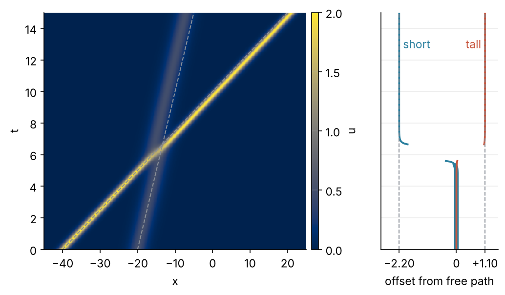
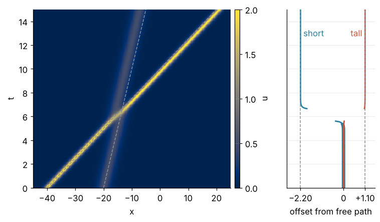
Left: u over x and t as a cividis image, with the tracks of a tall and a short soliton meeting near t = 6 and dashed lines for their free paths. Right: the offset of each track from its free path against t, settling at +1.10 for the tall one and −2.20 for the short one.

The space-time picture on the left shows the answer as a jog in each track against its dashed free path, and the right panel measures it: the tall soliton comes out 1.10 ahead, the short one 2.20 behind. It takes about 3 s on a laptop. Three pieces make it work: derivatives by the FFT, which the Fourier transform tutorial prepares, the 2/3 rule against aliasing in the product \(u^2\), and an integrating factor that removes the stiff third derivative before solve_ivp steps the rest. Step 6 draws the figure.

Setup

No data to load: the initial condition is the sum of two soliton formulas. Everything is in the equation's scaled units, so the axes carry none. The grid leaves out x = 50, which on a periodic domain is x = −50 again. The second number printed, grid points across the tall soliton, is the one Step 6 turns into a rule for N.

import numpy as np
import matplotlib.pyplot as plt
from numpy.fft import rfft, irfft, rfftfreq
from scipy.integrate import solve_ivp
from scipy.signal import find_peaks

L, N = 100.0, 512             # periodic domain [-50, 50), grid points
c1, c2 = 4.0, 1.0             # speeds of the tall and the short soliton
x1, x2 = -40.0, -20.0         # their starting positions
T = 15.0                      # end of the run

def soliton(x, c, x0):
    return 0.5 * c / np.cosh(0.5 * np.sqrt(c) * (x - x0))**2

x = -L / 2 + L * np.arange(N) / N
dx = L / N

plt.rcParams.update({
    "figure.figsize": (7, 3.6), "figure.dpi": 110,
    "axes.spines.top": False, "axes.spines.right": False,
    "axes.grid": True, "grid.alpha": 0.25,
    "font.size": 11, "lines.linewidth": 1.8,
})
INK, ACCENT, SECOND, MUTED = "#1f2a44", "#c8553d", "#2a7f9e", "#8a8f98"

width = 2 * np.arccosh(np.sqrt(2)) / (np.sqrt(c1) / 2)    # tall soliton at half height
print(f"dx = {dx:.3f}, {width / dx:.1f} grid points across the tall soliton's half-height width {width:.2f}")

dx = 0.195, 9.0 grid points across the tall soliton's half-height width 1.76

Step 1: Differentiate on a periodic grid with the FFT

A periodic function is a sum of waves \(e^{ikx}\), and differentiating one multiplies it by \(ik\). So a derivative is a transform, a multiplication by \(ik\), and a transform back. rfftfreq returns cycles per unit length, as in the Fourier transform tutorial; the factor 2π turns them into radians. Since u is real, rfft keeps only the 257 nonnegative wavenumbers. With norm="forward" the coefficients are amplitudes in units of u, independent of N. That pays off twice: atol means the same at every N, and zero-padding in Step 5 needs no rescaling.

The tall soliton's derivatives are known in closed form, with \(a = \sqrt c/2\), \(S = \mathrm{sech}^2 ax\) and \(\tau = \tanh ax\):

k = 2 * np.pi * rfftfreq(N, d=L / N)

a = np.sqrt(c1) / 2
S, tau = 1 / np.cosh(a * x)**2, np.tanh(a * x)
u = soliton(x, c1, 0.0)
ux_exact = -c1 * a * S * tau
uxxx_exact = -4 * c1 * a**3 * S * tau * (1 - 3 * S)

uh = rfft(u, norm="forward")
ux = irfft(1j * k * uh, n=N, norm="forward")
uxxx = irfft((1j * k)**3 * uh, n=N, norm="forward")
ux_fd = (np.roll(u, -1) - np.roll(u, 1)) / (2 * dx)      # second-order centered difference
print(f"FFT:                 max error u_x {np.abs(ux - ux_exact).max():.1e}, "
      f"u_xxx {np.abs(uxxx - uxxx_exact).max():.1e}")
print(f"centered difference: max error u_x {np.abs(ux_fd - ux_exact).max():.1e}")

FFT:                 max error u_x 7.3e-09, u_xxx 1.9e-06
centered difference: max error u_x 5.1e-02

Seven orders of magnitude separate the FFT from a second-order difference like those of the leapfrog tutorial on the same grid. For a smooth periodic function the coefficients fall off exponentially with k, and the error falls with them once the grid holds them all. That is called spectral accuracy.

Step 2: Write KdV as ODEs for the Fourier coefficients

Write \(6uu_x\) as \(3(u^2)_x\) and transform the equation. Every coefficient gets its own ODE,

\[\frac{d\hat u_k}{dt} = ik^3\,\hat u_k - 3ik\,\mathcal F[u^2]_k ,\]

257 complex ODEs that solve_ivp integrates like any system. Every equation this method handles has the same form,

\[\frac{d\hat u}{dt} = \mathcal L(k)\,\hat u + \hat N(u) .\]

\(\mathcal L(k)\) is the linear symbol, the number by which the linear terms multiply mode k on their own. With \(\partial_x \to ik\), KdV's \(u_t = -u_{xxx}\) gives \(\mathcal L(k) = -(ik)^3 = ik^3\). \(\hat N(u)\) is the nonlinear term, computed on the grid and transformed, here \(-3ik\,\mathcal F[u^2]\).

The argument keep is a mask that Step 3 fills in; here it keeps every mode. A single soliton satisfies \(u_t = -cu_x\), so the right-hand side evaluated on it must return \(-c\,ik\,\hat u\):

def rhs_direct(t, uh, k, keep):
    u = irfft(uh, n=2 * (len(uh) - 1), norm="forward")
    return 1j * k**3 * uh - 3j * k * keep * rfft(u * u, norm="forward")

def residual(x, k, keep):
    uh = keep * rfft(soliton(x, c1, 0.0), norm="forward")
    err = rhs_direct(0.0, uh, k, keep) - (-c1 * 1j * k * uh)   # exact u_t = -c u_x
    return np.abs(irfft(err, n=len(x), norm="forward")).max()

keep_all = np.ones_like(k, dtype=bool)
print(f"residual {residual(x, k, keep_all):.1e}, max |u_t| {np.abs(c1 * ux_exact).max():.2f}")
print(f"|û| at the highest wavenumber {abs(uh[-1]):.1e}, k_max³ = {k[-1]**3:.0f}")

residual 1.8e-07, max |u_t| 6.09
|û| at the highest wavenumber 4.3e-11, k_max³ = 4162

A residual of 2 × 10⁻⁷ against a \(u_t\) of 6. The cause is on the screen: the soliton's coefficient at the grid's highest wavenumber is 4 × 10⁻¹¹, and the \(k^3\) term multiplies it by 4,162. That is the grid's truncation. A wrong sign or factor would give a residual of order one.

Step 3: Dealias the product with the 2/3 rule

If u holds wavenumbers up to \(k_{\max} = \pi N/L\), its square holds them up to \(2k_{\max}\), and the grid cannot represent anything above \(k_{\max}\). By the folding of the Fourier transform tutorial, a mode at \(k > k_{\max}\) shows up at \(2k_{\max} - k\), wrong energy in a mode the solver keeps. On 16 points in index units, \(k_{\max} = 8\):

xj = 2 * np.pi * np.arange(16) / 16
for name, f in [("cos 5x cos 6x", np.cos(5 * xj) * np.cos(6 * xj)),
                ("cos 5x cos 5x", np.cos(5 * xj)**2)]:
    print(f"{name}: modes {np.flatnonzero(np.abs(rfft(f)) > 1e-9)}")

cos 5x cos 6x: modes [1 5]
cos 5x cos 5x: modes [0 6]

The first product should hold modes 1 and 11, and 11 lands on 16 − 11 = 5. The cure is to keep only \(k < k_c\), in the state and in \(\hat N\). A product of two kept modes then has \(k < 2k_c\), and it folds to

\[2k_{\max} - k > 2k_{\max} - 2k_c \ge k_c \quad\text{when}\quad k_c \le \tfrac23\,k_{\max} ,\]

among the discarded modes. That is the 2/3 rule. Here the cutoff is 16/3 ≈ 5.3, so a dealiased state never holds cos 6x, and the second product's mode 10 folds to 6, just above the cutoff: discarded.

def grid(N):
    x = -L / 2 + L * np.arange(N) / N
    k = 2 * np.pi * rfftfreq(N, d=L / N)
    keep = k < 2 / 3 * k.max()
    return x, k, keep

for n in [512, 768]:
    xn, kn, keep = grid(n)
    cut = keep.sum()                                # index of the first discarded mode
    uh_cut = abs(rfft(soliton(xn, c1, 0.0), norm="forward")[cut])
    print(f"N = {n}: {cut} of {kn.size} modes kept, residual {residual(xn, kn, keep):.1e}, "
          f"|û| at the cutoff {uh_cut:.0e}")

N = 512: 171 of 257 modes kept, residual 5.0e-05, |û| at the cutoff 6e-08
N = 768: 256 of 385 modes kept, residual 2.6e-08, |û| at the cutoff 2e-11

In one evaluation the mask costs accuracy, 5 × 10⁻⁵ against Step 2's 2 × 10⁻⁷, because the products miss the coefficients of 6 × 10⁻⁸ at the cutoff. At 768 the cost is down to 3 × 10⁻⁸. What the rule prevents builds up over a run: each step folds a little energy into kept modes, and the next product folds it again. KdV conserves \(\int u^2\,dx\), the masked equations do so exactly, and by Parseval a fixed value bounds every coefficient. Without the mask nothing does. Step 5 and the first pitfall show both sides.

Step 4: Take the stiff k³ term out with an integrating factor

First the problem, measured. RK45 accepts a complex state, so the coefficients go to solve_ivp unchanged. The linear term spins mode k at frequency \(k^3\), and an explicit method must follow the fastest spin to stay stable: its step shrinks like \(k_c^{-3}\), and doubling N costs a factor of 8.

The linear part alone has the exact solution \(\hat u = e^{\mathcal L(k)t}\,\hat u(0)\). Substitute \(\hat v = e^{-\mathcal L(k)t}\,\hat u\) and the linear term drops out:

\[\frac{d\hat v}{dt} = e^{-\mathcal L(k)t}\,\hat N(u), \qquad u = \mathcal F^{-1}\big[e^{\mathcal L(k)t}\,\hat v\big] ,\]

with \(e^{-ik^3t}\) for KdV. The fast rotation now multiplies only the nonlinear term, and \(\hat N\) changes with \(\hat v\) at a rate of about \(6\max|u|\,k\), the advection by 6u, not \(k^3\). The rotation is fastest near the cutoff, where \(\hat N\) is tiny, so RK45 can follow it loosely without losing accuracy. The factor can run from t = 0 to the end because KdV's imaginary symbol keeps its modulus at one; a damping term, as in viscous Burgers, makes it grow until it overflows (Variations).

def rhs_if(t, v, k, keep):
    E = np.exp(1j * k**3 * t)                       # e^{L(k) t}
    u = irfft(E * v, n=2 * (len(v) - 1), norm="forward")
    return keep * np.conj(E) * (-3j * k * rfft(u * u, norm="forward"))

print("    N   direct nfev   factor nfev    k_c³")
for n in [256, 512, 1024]:
    xn, kn, keep = grid(n)
    uh0 = keep * rfft(soliton(xn, c1, x1) + soliton(xn, c2, x2), norm="forward")
    direct, factor = [solve_ivp(rhs, (0, 2), uh0, args=(kn, keep), rtol=1e-8, atol=1e-10)
                      for rhs in (rhs_direct, rhs_if)]
    print(f"{n:5d} {direct.nfev:13,d} {factor.nfev:13,d} {kn[keep].max()**3:7,.0f}")

    N   direct nfev   factor nfev    k_c³
  256         3,104         3,524     152
  512        10,904         5,180   1,219
 1024       108,452         5,066   9,836

Without the factor the count grows 9.9-fold from 512 to 1024, near the predicted 8, against 4 for the \(\Delta x^2\) step limit of the heat equation. With the factor the count is flat from 512 on: accuracy sets the step, as it does for both at 256, so the direct count grows only 3.5-fold to 512.

Radau and LSODA, the solvers the solve_ivp tutorial recommends for a stiff problem, refuse a complex state. The integrating factor instead solves the linear, diagonal stiff term exactly. For KdV with RK45 that removes the stiffness, as the table shows.

Step 5: Run the collision and measure the shifts

solve masks the initial coefficients, runs rhs_if with output at 301 times, and turns \(\hat v\) back into \(\hat u\). Step 6 and the pitfalls reuse it.

def solve(N, T=T, rtol=1e-8, atol=1e-10, x1=x1, dealias=True):
    x, k, keep = grid(N)
    if not dealias:
        keep = np.ones_like(keep)
    uh0 = keep * rfft(soliton(x, c1, x1) + soliton(x, c2, x2), norm="forward")
    t = np.linspace(0, T, round(20 * T) + 1)
    sol = solve_ivp(rhs_if, (0, T), uh0, t_eval=t, args=(k, keep), rtol=rtol, atol=atol)
    Uh = sol.y.T * np.exp(1j * np.outer(sol.t, k**3))
    return sol.t, x, Uh, sol

t, x, Uh, sol = solve(N)
U = irfft(Uh, n=N, norm="forward", axis=1)
int_u2 = (U**2).sum(axis=1) * dx
print(f"nfev = {sol.nfev:,}, largest relative change of ∫u² dx: {np.abs(int_u2 - int_u2[0]).max() / int_u2[0]:.1e}")

nfev = 37,088, largest relative change of ∫u² dx: 3.3e-08

The masked equations conserve \(\int u^2\,dx\) (Step 3), so the drift of 3 × 10⁻⁸ is the time stepping's alone.

fig, ax = plt.subplots()
for t_snap, alpha in zip([0, 5, 6, 7, 15], [0.3, 0.45, 0.6, 0.8, 1.0]):
    i = round(t_snap / t[1])
    ax.plot(x, U[i], color=ACCENT, alpha=alpha)
    ax.text(x[U[i].argmax()], U[i].max() + 0.08, f"t = {t_snap}", color=ACCENT,
            alpha=0.55 + 0.45 * alpha, ha="center")
ax.set(xlabel="x", ylabel="u", xlim=(-45, 30), ylim=(-0.1, 2.4))
plt.show()
print(f"highest point at t = 6: {U[round(6 / t[1])].max():.2f}")

u against x at t = 0, 5, 6, 7, and 15, darker with time. At t = 6 the two solitons have merged into a single hump lower than the tall soliton; at t = 7 the tall one is in front again.

highest point at t = 6: 1.54

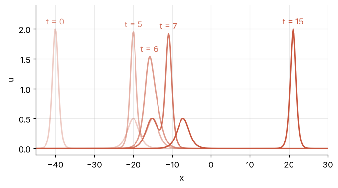
At t = 6 there is one hump, 1.54 high, lower than the tall soliton alone. By t = 7 the tall one is in front again.

The shifts need peak positions to better than the grid spacing of 0.195. Appending zero coefficients evaluates the same sum of \(e^{ikx}\) at 16 times more points. find_peaks returns the indices of the local maxima above height, and a parabola through the top three points places each between them. The shift is \(x_{\text{peak}} - (x_0 + cT)\). With \(\kappa = \sqrt c/2\), so \(\kappa_1 = 1\) and \(\kappa_2 = 1/2\), the two-soliton solution of KdV moves the fast one forward and the slow one back by

\[\delta_1 = \frac{1}{\kappa_1}\ln\frac{\kappa_1 + \kappa_2}{\kappa_1 - \kappa_2} = \ln 3, \qquad \delta_2 = \frac{1}{\kappa_2}\ln\frac{\kappa_1 + \kappa_2}{\kappa_1 - \kappa_2} = 2\ln 3 .\]

def peaks(uh, N, pad=16):
    n = pad * N
    uf = irfft(uh, n=n, norm="forward")             # the same series at 16 times more points
    xf = -L / 2 + L * np.arange(n) / n
    found = []
    for i in find_peaks(uf, height=0.2)[0]:
        ym, y0, yp = uf[i - 1], uf[i], uf[(i + 1) % n]
        d = 0.5 * (ym - yp) / (ym - 2 * y0 + yp)    # vertex of the parabola, in fine steps
        found.append((xf[i] + d * L / n, y0 - 0.25 * (ym - yp) * d))
    return sorted(found, key=lambda p: -p[1])       # (position, height), tallest first

def shifts(Uh, N, x1=x1):
    (xa, _), (xb, _) = peaks(Uh[-1], N)[:2]
    return xa - (x1 + c1 * T), xb - (x2 + c2 * T)

shift_tall, shift_short = shifts(Uh, N)
print(f"tall:  shift {shift_tall:+.6f}, exact +ln 3   = {np.log(3):+.6f}")
print(f"short: shift {shift_short:+.6f}, exact -2 ln 3 = {-2 * np.log(3):+.6f}")

tall:  shift +1.098612, exact +ln 3   = +1.098612
short: shift -2.197225, exact -2 ln 3 = -2.197225

Both shifts agree with the exact values to the six decimals printed.

Step 6: Check the number of modes and draw the collision

Rerun at 256, 384, and 768 points, and once at 512 with solve_ivp's default tolerances:

results = {N: (shift_tall, shift_short)}
for n in [256, 384, 768]:
    results[n] = shifts(solve(n)[2], n)
print("    N   tall shift    error   short shift    error")
for n in sorted(results):
    st, ss = results[n]
    print(f"{n:5d} {st:+12.6f} {abs(st - np.log(3)):8.1e} {ss:+13.6f} {abs(ss + 2 * np.log(3)):8.1e}")

_, _, Uh_d, sol_d = solve(N, rtol=1e-3, atol=1e-6)
st, ss = shifts(Uh_d, N)
print(f"N = {N}, default tolerances: shifts {st:+.4f} and {ss:+.4f}, nfev = {sol_d.nfev:,}")

    N   tall shift    error   short shift    error
  256    +1.086428  1.2e-02     -2.200469  3.2e-03
  384    +1.098590  2.3e-05     -2.197325  1.0e-04
  512    +1.098612  5.4e-07     -2.197225  4.3e-07
  768    +1.098612  2.2e-07     -2.197223  1.9e-06
N = 512, default tolerances: shifts +1.0097 and -2.1229, nfev = 5,288

From 256 to 384 points the error of the tall shift falls from 1.2 × 10⁻² to 2.3 × 10⁻⁵, a factor of 500 for 50 % more modes. That is exponential convergence; the leapfrog scheme gains a factor of 4 per halving of the spacing. At 768 nothing more is gained. With the default tolerances the tall shift is 8 % low. For your own problem, put about 9 grid points across the half-height width of the narrowest feature, keep the 2/3 rule, and confirm with one run at 1.5 times as many points.

The final figure needs each peak's offset from its free track at every output time:

offset = np.full((len(t), 2), np.nan)               # tall, short; NaN while there is one hump
for i, (ti, uh_i) in enumerate(zip(t, Uh)):
    found = peaks(uh_i, N)
    if len(found) == 2:
        offset[i] = found[0][0] - (x1 + c1 * ti), found[1][0] - (x2 + c2 * ti)
one_hump = t[np.isnan(offset[:, 0])]

fig = plt.figure(figsize=(8, 4.2))
gs = fig.add_gridspec(1, 4, width_ratios=[2.8, 0.07, 0.55, 1.25], wspace=0.05)  # image, colorbar, gap, offsets
ax, cax = fig.add_subplot(gs[0]), fig.add_subplot(gs[1])
ax2 = fig.add_subplot(gs[3], sharey=ax)
im = ax.pcolormesh(x, t, U, cmap="cividis", shading="auto", vmin=0, vmax=2, rasterized=True)
for x0, c in [(x1, c1), (x2, c2)]:
    ax.plot(x0 + c * t, t, color=MUTED, lw=1, ls="--")
fig.colorbar(im, cax=cax, ticks=[0, 0.5, 1, 1.5, 2]).set_label("u", labelpad=2)
ax.set(xlabel="x", ylabel="t", xlim=(-45, 25), ylim=(0, T))
ax.grid(False)
both = np.abs(offset[:, 0] - offset[:, 1]) < 0.05   # before the collision both offsets are 0
ax2.plot(np.where(both, offset[:, 1], np.nan), t, color=SECOND, lw=4.5)   # short, wide under the tall
ax2.plot(offset[:, 1], t, color=SECOND)
ax2.plot(offset[:, 0], t, color=ACCENT)
for value in [np.log(3), -2 * np.log(3)]:
    ax2.axvline(value, color=MUTED, lw=1, ls="--")
ax2.text(-2.05, 13, "short", color=SECOND, ha="left", va="center")
ax2.text(0.95, 13, "tall", color=ACCENT, ha="right", va="center")
ax2.set_xticks([-2 * np.log(3), 0, np.log(3)], ["−2.20", "0", "+1.10"])
ax2.grid(False, axis="x")
ax2.tick_params(labelleft=False, left=False)
ax2.set(xlabel="offset from free path", xlim=(-2.9, 1.6))
plt.show()
print(f"one hump from t = {one_hump.min():.2f} to {one_hump.max():.2f}")

Left: u over x and t as a cividis image, with the tracks of a tall and a short soliton meeting near t = 6 and dashed lines for their free paths. Right: the offset of each track from its free path against t, settling at +1.10 for the tall one and −2.20 for the short one.

one hump from t = 5.65 to 6.60

Each bright track jogs against its dashed free path, and the offsets settle on the exact values. The gap in the offset curves is the single hump, from t = 5.65 to 6.60, slightly before the free tracks cross.

Pitfalls

Leaving out the 2/3 rule. At 128 points the tall soliton's half-height width spans about 2.3 grid points. Run it to t = 30 with and without the mask:

for dealias in [False, True]:
    t_p, _, Uh_p, sol_p = solve(128, T=30.0, dealias=dealias)
    U_p = irfft(Uh_p, n=128, norm="forward", axis=1)
    I_p = (U_p**2).sum(axis=1)
    print(f"2/3 rule {'on ' if dealias else 'off'}: status {sol_p.status:2d}, last output t = {t_p[-1]:4.1f}, "
          f"max |u| {np.abs(U_p).max():5.1f}, largest change of ∫u² dx {np.abs(I_p - I_p[0]).max() / I_p[0]:.1e}")
print("heights at t = 30 with the rule:", ", ".join(f"{h:.2f}" for _, h in peaks(Uh_p[-1], 128)))

2/3 rule off: status -1, last output t =  5.2, max |u| 133.5, largest change of ∫u² dx 7.1e+03
2/3 rule on : status  0, last output t = 30.0, max |u|   1.9, largest change of ∫u² dx 5.9e-07
heights at t = 30 with the rule: 1.82, 0.50

Without the mask the solver gives up after t = 5.2, with max |u| at 133.5 and \(\int u^2\,dx\) grown about 7,000-fold. With it the run reaches t = 30, the integral drifts by 6 × 10⁻⁷, and the tall soliton is 1.82 high instead of 2. The rule turns an explosion into an inaccuracy, and the cure for the inaccuracy is more modes (Step 6). A conserved \(\int u^2\,dx\) proves nothing about accuracy in a dealiased run, since the mask conserves it by construction.

Wavenumbers in the wrong units or order. rfftfreq without the 2π makes \(u_x\) too small by 2π and \(u_{xxx}\) by (2π)³ ≈ 248. The equation is then nearly dispersionless, and the solitons steepen and break into a train of peaks instead of keeping their shape. With the full fft, writing k = 2*np.pi/L*np.arange(N) instead of using fftfreq gives the upper half of the modes positive wavenumbers that belong negative, and the derivative of a real function an imaginary part larger than the derivative itself. Taking .real throws away the evidence, not the error. The fix is Step 1's check on a function with a known derivative, every time the grid changes.

Solitons started too close, or a domain too short. The sum of two solitons is a two-soliton state only when they are far apart, since the short one's tail at distance d is about \(2e^{-d}\). Start the tall one 10, 15, and 20 behind the short one on the same domain:

Show code

for sep in [10, 15, 20]:
    st, ss = shifts(solve(N, x1=x2 - sep)[2], N, x1=x2 - sep)
    print(f"started {sep} apart: tall shift {st:+.6f}, short shift {ss:+.6f}")

started 10 apart: tall shift +1.106926, short shift -2.197079
started 15 apart: tall shift +1.098668, short shift -2.197223
started 20 apart: tall shift +1.098612, short shift -2.197225

At 10 apart the tall shift is 0.8 % high; at 20 it is exact to the printed digits. On a periodic domain the fast soliton also laps the slow one every \(L/(c_1 - c_2)\) = 100/3 ≈ 33 time units, so a second collision comes near t ≈ 40 here. Start them at least 20 apart, and end the run before the next lap.

Variations

Three solitons. Add a c = 9 soliton behind the other two. Each soliton's total shift is the sum of its pairwise shifts, and N must grow, because the new one is 1.5 times narrower than the tall one (the rule of Step 6).
A hump that is not a soliton. Start from \(u_0 = 6\,\mathrm{sech}^2 x\). It breaks into exactly two solitons, of heights 8 and 2 and speeds 16 and 4. The integrating factor matters more here, since the narrower soliton needs more modes and the direct step limit tightens with their cube.
Other equations, same split. For the nonlinear Schrödinger equation \(i\psi_t + \psi_{xx} + 2|\psi|^2\psi = 0\) the symbol is \(\mathcal L(k) = -ik^2\), so the factor is \(e^{ik^2t}\); the full fft replaces rfft, because ψ is complex; and the cubic term needs \(k_c \le k_{\max}/2\) by Step 3's argument with three factors. A symbol with a negative real part makes Step 4's factor grow, as \(e^{\nu k^2 t}\) for viscous Burgers and \(e^{(k^4 - k^2)t}\) for Kuramoto-Sivashinsky, \(\mathcal L(k) = k^2 - k^4\), and it overflows once the exponent at \(k_{\max}\) passes 709.8, the natural logarithm of the largest float64. To run longer, restart the factor at every step of a Runge-Kutta loop of your own, as Trefethen's program 27 does for KdV. That is the integrating-factor Runge-Kutta method. Kassam and Trefethen find that it works well for Burgers and set it against exponential time differencing (ETDRK4).
Walls instead of periodicity. Fourier modes need periodic boundaries. A wall needs another basis, such as Chebyshev polynomials, which a tutorial planned on this site will cover.

Cheat sheet

x = -L/2 + L*np.arange(N)/N                     # periodic: no endpoint
k = 2*np.pi*rfftfreq(N, d=L/N)                  # angular wavenumbers, not cycles
keep = k < 2/3*k.max()                          # folds land at 2 k_max - k, all discarded
F = lambda u: rfft(u, norm="forward")           # coefficients in units of u
Finv = lambda uh: irfft(uh, n=N, norm="forward")
def rhs(t, v):                                  # v = e^{-L(k) t} û with L(k) = i k^3
    E = np.exp(1j*k**3*t)
    return keep*np.conj(E)*(-3j*k*F(Finv(E*v)**2))
sol = solve_ivp(rhs, (0, T), keep*F(u0), rtol=1e-8, atol=1e-10)
u_T = Finv(np.exp(1j*k**3*T)*sol.y[:, -1])      # check N with one run at 1.5 N