Gerchberg-Saxton algorithm in NumPy: a phase-only hologram for 25 spots

The problem: which phase mask turns a laser beam into 25 spots?

Optical tweezers hold a bead or a cell in the focus of a laser beam. To hold 25 of them you need 25 foci, and the usual way to make them is a spatial light modulator (SLM): a liquid-crystal screen, here 512 × 512 pixels, that delays the phase of the beam pixel by pixel and leaves its amplitude alone. Behind a lens, the focal plane holds the two-dimensional Fourier transform of the field on the SLM; take that as a premise, which the angular spectrum tutorial and Goodman (Further reading) back up. Which phase mask puts the light into a 5 × 5 array of spots?

No formula gives it. On the SLM you know the amplitude, the Gaussian profile of the laser, and choose the phase. In the focal plane you know the amplitude you want and leave the phase free. The Gerchberg-Saxton algorithm (GS) goes back and forth between the two planes with fft2 and ifft2, keeps the phase it computed each time, and replaces the amplitude by the known one. The error in the focal plane never rises from one round to the next. Designing a hologram is phase retrieval with a target you chose instead of one you measured, and the same loop recovers phases from measured intensities in electron microscopy, X-ray coherent diffraction imaging, and, in a variant fed with several defocused images, the wavefront sensing that aligned the 18 mirror segments of the James Webb Space Telescope.

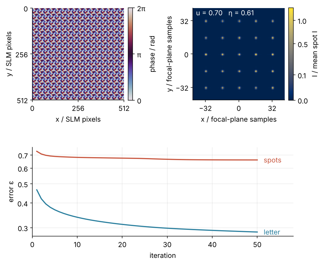
Left: an 8-bit phase mask of 512 by 512 SLM pixels, a woven pattern repeating every 32 pixels. Right: the focal-plane intensity it makes, a 5 by 5 grid of spots, uniformity 0.70. Bottom: error against iteration on a log axis for the spots and for a letter F; the letter ends lower.

Top left is the 8-bit phase mask, which looks nothing like spots. Top right are the 25 spots it makes after 50 iterations, with 61 % of the light in them and a uniformity of 0.70, where 1 means 25 equal spots. At the bottom is the error of each round, for the spots and for a letter F. Step 6 draws the figure.

Setup

The SLM has 8 µm pixels, the laser is the 1064 nm infrared common in tweezers, and the lens has a focal length of 200 mm. The beam is a Gaussian centered on the screen.

The discrete transform of \(N\) pixels of size \(\Delta x\), pitch in the code, has frequencies spaced \(1/(N\Delta x)\) apart, and the lens puts the spatial frequency \(\nu\) at the focal position \(\lambda f \nu\). One focal-plane sample is therefore \(\lambda f/(N\Delta x)\), the unit of every position below; to place your own traps, divide their spacing in µm by it. The square screen also cuts off the tails of the Gaussian, so the cell checks how much power that loses.

import numpy as np
import matplotlib.pyplot as plt

N = 512                       # SLM pixels per side
pitch = 8e-6                  # m
wavelength = 1064e-9          # m
f = 0.2                       # m, focal length of the Fourier lens
w = 0.35 * N * pitch          # m, beam radius

plt.rcParams.update({
    "figure.figsize": (7, 3.6), "figure.dpi": 110,
    "axes.spines.top": False, "axes.spines.right": False,
    "axes.grid": True, "grid.alpha": 0.25,
    "font.size": 11, "lines.linewidth": 1.8,
})
INK, ACCENT, SECOND, MUTED = "#1f2a44", "#c8553d", "#2a7f9e", "#8a8f98"

rng = np.random.default_rng(286)            # Step 2 draws the start phase from it

x = (np.arange(N) - N // 2) * pitch
X, Y = np.meshgrid(x, x)
A = np.exp(-(X**2 + Y**2) / w**2)           # beam amplitude on the SLM

sample = wavelength * f / (N * pitch)
clipped = 1 - np.sum(A**2) / (np.pi * w**2 / 2 / pitch**2)   # against the unclipped Gaussian
print(f"beam radius {w * 1e3:.2f} mm, one focal-plane sample = {sample * 1e6:.1f} µm")
print(f"power clipped by the square SLM: {clipped:.2%}")

beam radius 1.43 mm, one focal-plane sample = 52.0 µm
power clipped by the square SLM: 0.85%

One sample is 52.0 µm, and 0.85 % of the power falls off the screen, too little to change any number below.

Step 1: Build the targets inside a dark border

The first target is 25 single samples, 16 samples apart, centered on the axis. The second is a letter F, 120 samples tall, built from three rectangles so that it needs no font. An F also shows at a glance whether the picture came out mirrored. match_power scales each target to the power of the beam.

c = N // 2
offsets = np.arange(-32, 33, 16)
T_spots = np.zeros((N, N))
T_spots[np.ix_(c + offsets, c + offsets)] = 1

def letter_F(height, width, stroke):
    T = np.zeros((N, N))
    top, left = c - height // 2, c - width // 2
    middle = top + height // 2 - stroke // 2
    T[top:top + height, left:left + stroke] = 1               # the stem
    T[top:top + stroke, left:left + width] = 1                # the top bar
    T[middle:middle + stroke, left:left + 2 * width // 3] = 1 # the middle bar
    return T

def match_power(T):
    return T * np.sqrt(np.sum(A**2) / np.sum(T**2))

T_spots = match_power(T_spots)
T_F = match_power(letter_F(120, 60, 20))
print(f"spot samples: {np.count_nonzero(T_spots)}, letter samples: {np.count_nonzero(T_F)}")
print(f"power: beam {np.sum(A**2):.1f}, spots {np.sum(T_spots**2):.1f}, letter {np.sum(T_F**2):.1f}")

spot samples: 25, letter samples: 3600
power: beam 50012.0, spots 50012.0, letter 50012.0

Both targets carry exactly the power of the beam, a sum of squared amplitudes of 50012.0. The transforms below use norm="ortho", which scales fft2 and ifft2 so that the sum of \(|E|^2\) is the same before and after, Parseval's theorem from the prerequisite. A target with the beam's power is one the light can actually fill, and the error defined in Step 2 has a fixed scale.

Both patterns also stay within the central 256 × 256 samples. The focal window is periodic, because the discrete transform repeats every \(N\) samples and so does the light behind a pixelated SLM. A real SLM also puts a bright spot on the axis that has to be moved out of the way, and the dark border is the room to shift the pattern 64 samples off the axis without wrapping it around the edge (the first two pitfalls).

Step 2: Write the Gerchberg-Saxton loop

One round of GS is four operations. Put the beam amplitude and the current phase together on the SLM and transform to the focal plane. Keep the phase you find there and replace the amplitude by the target. Transform back to the SLM. Keep the phase you find there; its amplitude is replaced by the beam's at the start of the next round.

The loop needs a phase before the first transform, and nothing is known about it. The usual choice is a uniformly random phase, phi0, which spreads the light over the whole focal plane from the start. The result depends on this guess, the third pitfall shows by how much, and drawing it from the seeded rng makes every number below reproducible.

The targets have their center at index \(N/2\), while NumPy's transform puts zero frequency at index 0. So ifftshift moves the center to index 0 before fft2, and fftshift moves it back after (the MRI tutorial has more on the order).

def to_focal(E):
    return np.fft.fftshift(np.fft.fft2(np.fft.ifftshift(E), norm="ortho"))

def to_slm(F):
    return np.fft.fftshift(np.fft.ifft2(np.fft.ifftshift(F), norm="ortho"))

def gerchberg_saxton(A, T, phi0, n_iter):
    on = T > 0
    err, eff = [], []
    F = to_focal(A * np.exp(1j * phi0))
    for _ in range(n_iter):
        phi = np.angle(to_slm(T * np.exp(1j * np.angle(F))))
        F = to_focal(A * np.exp(1j * phi))
        amp = np.abs(F)                    # measured before the target is imposed again
        err.append(np.sqrt(np.sum((amp - T) ** 2) / np.sum(T**2)))
        eff.append(np.sum(amp[on] ** 2) / np.sum(amp**2))
    return phi, np.array(err), np.array(eff)

def focal_intensity(A, phi):
    return np.abs(to_focal(A * np.exp(1j * phi))) ** 2

def uniformity(I):
    return 1 - (I.max() - I.min()) / (I.max() + I.min())

phi0 = rng.uniform(0, 2 * np.pi, A.shape)
_, err1, eff1 = gerchberg_saxton(A, T_spots, phi0, 1)
print(f"after one round: error {err1[0]:.3f}, efficiency {eff1[0]:.3f}")

after one round: error 0.731, efficiency 0.550

The function records two numbers per round. The error \(\varepsilon = \sqrt{\sum(|F| - T)^2 / \sum T^2}\) compares the focal amplitude \(|F|\) with the target \(T\); Fienup proved that this quantity, taken before the target is imposed, never rises. The efficiency \(\eta\) is the fraction of the power that lands on the target samples. After one round, 55 % of the light is already in the 25 spots.

Step 3: Run it for 25 spots and measure efficiency and uniformity

The cell runs fifty rounds from the same start phase and then checks three things. First, whether the error ever rises, and the floor that the light missing the spots puts under it. Second, whether that light lies far away or next to the spots: near marks every sample within one sample of a spot center, and I_lens, the beam focused through a flat mask, shows the most one focus can put into a single sample. Third, how equal the 25 spots are.

phi_spots, err_spots, eff_spots = gerchberg_saxton(A, T_spots, phi0, 50)
for k in [1, 2, 5, 10, 20, 50]:
    print(f"iteration {k:2d}   error {err_spots[k - 1]:.4f}   efficiency {eff_spots[k - 1]:.4f}")
print("error never rises:", np.all(np.diff(err_spots) <= 1e-12))
print(f"error floor from the light off target, sqrt(1 - efficiency): {np.sqrt(1 - eff_spots[-1]):.4f}")

on = T_spots > 0
I = focal_intensity(A, phi_spots)
I_spot = I[on]
near = np.any([np.roll(on, (di, dj), axis=(0, 1)) for di in (-1, 0, 1) for dj in (-1, 0, 1)], axis=0)
I_lens = focal_intensity(A, np.zeros_like(A))          # flat mask: the beam focused to one spot
print(f"power within one sample of a spot center: {I[near].sum() / I.sum():.3f}")
print(f"power a single focused spot puts into its brightest sample: {I_lens.max() / I_lens.sum():.3f}")
print(f"spot intensity / mean: min {I_spot.min() / I_spot.mean():.3f}, max {I_spot.max() / I_spot.mean():.3f}")
print(f"uniformity u = {uniformity(I_spot):.3f}")

iteration  1   error 0.7310   efficiency 0.5501
iteration  2   error 0.7086   efficiency 0.5705
iteration  5   error 0.6889   efficiency 0.5893
iteration 10   error 0.6812   efficiency 0.5981
iteration 20   error 0.6751   efficiency 0.6028
iteration 50   error 0.6610   efficiency 0.6143
error never rises: True
error floor from the light off target, sqrt(1 - efficiency): 0.6210
power within one sample of a spot center: 0.944
power a single focused spot puts into its brightest sample: 0.650
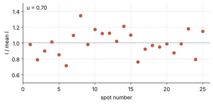
spot intensity / mean: min 0.716, max 1.343
uniformity u = 0.696

The error falls fastest in the first five rounds, from 0.731 to 0.689, and creeps down to 0.661 by round 50. Most of what is left is the light off target: since target and focal field carry the same power, the 39 % of the light that misses the 25 samples alone gives \(\varepsilon \geq \sqrt{1 - \eta} = 0.621\). That light does not wander off: 94 % of the power lies within one sample of a spot center, so the spots are simply wider than one sample. They cannot be narrower: the beam focused by the lens alone, with no mask, puts only 65 % of its power into its brightest sample, and GS gets 61 %.

The spots themselves are unequal. The weakest has 72 % of the mean intensity, the strongest 134 %, and the uniformity \(u = 1 - (I_\max - I_\min)/(I_\max + I_\min)\), the measure of Di Leonardo and coworkers, is 0.696. In a tweezer array the weakest trap is the one that lets its bead go first.

fig, ax = plt.subplots(figsize=(7, 3))
ax.plot(np.arange(1, 26), I_spot / I_spot.mean(), "o", color=ACCENT, ms=6)
ax.axhline(1, color=MUTED, lw=1, ls="--")
ax.text(0.02, 0.92, f"u = {uniformity(I_spot):.2f}", transform=ax.transAxes)
ax.set(xlabel="spot number", ylabel="I / mean I", xlim=(0, 26), ylim=(0.5, 1.5))
plt.show()

Intensity of each of the 25 spots divided by the mean, against spot number 1 to 25, around a dashed line at 1. Values range from about 0.7 to 1.35; uniformity 0.70.

Step 4: Project the letter and look at the grain

The same function, the letter as target, and a fresh random start:

letter = T_F > 0
phi_F, err_F, eff_F = gerchberg_saxton(A, T_F, rng.uniform(0, 2 * np.pi, A.shape), 50)
I_F = focal_intensity(A, phi_F)

def contrast(I):
    return I[letter].std() / I[letter].mean()

print(f"letter after 50 rounds: error {err_F[-1]:.3f}, efficiency {eff_F[-1]:.3f}, contrast C = {contrast(I_F):.3f}")

letter after 50 rounds: error 0.285, efficiency 0.929, contrast C = 0.199

crop = np.s_[c - 96:c + 96, c - 96:c + 96]
extent = (-96, 96, -96, 96)
fig, axes = plt.subplots(1, 2, figsize=(7, 3.5), sharey=True)
for ax, img in zip(axes, [T_F**2, I_F]):
    ax.imshow(img[crop], cmap="cividis", extent=extent, vmin=0, vmax=2 * T_F.max() ** 2)   # one scale for both
    ax.set(xlabel="x / samples")
    ax.grid(False)
axes[0].set(ylabel="y / samples")
axes[1].text(-88, -88, f"C = {contrast(I_F):.2f}", color="white")
plt.show()

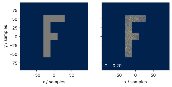
Two images of the central 192 by 192 focal-plane samples. Left: the target, a flat letter F. Right: the reconstruction, the same F with a fine grain of brighter and darker samples across it, speckle contrast 0.20.

The letter is there, sharp-edged, with 93 % of the light in it, and its intensity has a grain of brighter and darker samples. The speckle contrast \(C\), the standard deviation of the intensity over the letter divided by its mean, is 0.199. The cause is what a phase-only mask cannot do. Every SLM pixel contributes to the focal field with an amplitude the Gaussian beam fixes, and only its phase is free. A flat, sharp-edged letter would need a particular set of amplitudes as well, so GS settles on phases that come close, and the remainder shows up as grain inside the letter and light outside it.

The grain is the leftover of one particular solution, not a feature of the letter. A second start phase gives a different grain of the same strength, and four times as many rounds barely change it:

phi_F2, _, _ = gerchberg_saxton(A, T_F, rng.uniform(0, 2 * np.pi, A.shape), 50)
I_F2 = focal_intensity(A, phi_F2)
r = np.corrcoef(I_F[letter], I_F2[letter])[0, 1]
print(f"second start phase: C = {contrast(I_F2):.3f}, correlation with the first grain {r:.2f}")

phi_F200, _, _ = gerchberg_saxton(A, T_F, phi_F, 150)    # 150 more rounds, 200 in total
print(f"after 200 rounds: C = {contrast(focal_intensity(A, phi_F200)):.3f}")

second start phase: C = 0.203, correlation with the first grain 0.16
after 200 rounds: C = 0.185

Same contrast within 2 %, a correlation of 0.16 between the two grain patterns, and 150 more rounds take \(C\) from 0.199 to 0.185.

Step 5: Quantize the phase to 8 bits

A phase-only hologram such as this mask is called a kinoform, and a real SLM can only show it with a finite number of gray levels, usually 256 per \(2\pi\). Round the 50-round spot mask to \(M\) levels and measure again:

def quantize(phi, M):
    return np.round(np.mod(phi, 2 * np.pi) / (2 * np.pi) * M) % M * (2 * np.pi / M)

eta = I_spot.sum() / I.sum()
for M in [256, 16, 4]:
    Iq = focal_intensity(A, quantize(phi_spots, M))
    ratio = Iq[on].sum() / Iq.sum() / eta
    print(f"M = {M:3d}   efficiency ratio {ratio:.5f}   sinc²(1/M) {np.sinc(1 / M) ** 2:.5f}   u {uniformity(Iq[on]):.3f}")
phi_8bit = quantize(phi_spots, 256)
print("8-bit mask repeats every 32 pixels:",
      np.array_equal(phi_8bit, np.roll(phi_8bit, 32, axis=0)), np.array_equal(phi_8bit, np.roll(phi_8bit, 32, axis=1)))

M = 256   efficiency ratio 0.99994   sinc²(1/M) 0.99995   u 0.696
M =  16   efficiency ratio 0.98743   sinc²(1/M) 0.98721   u 0.685
M =   4   efficiency ratio 0.82876   sinc²(1/M) 0.81057   u 0.400
8-bit mask repeats every 32 pixels: True True

Rounding leaves each pixel with a phase error of up to half a step. The light that stays in the pattern is the average of \(e^{i\delta}\) over these errors \(\delta\), squared; for errors spread evenly over one step the average is \(\mathrm{sinc}(1/M)\), so the ratio is \(\mathrm{sinc}^2(1/M)\). Here sinc is the normalized \(\sin(\pi x)/(\pi x)\) that np.sinc computes, not the \(\sin(x)/x\) of many physics courses. At 256 and 16 levels the measured ratio matches it within 0.0003; at four levels 17 % of the light leaves the pattern, and the uniformity drops from 0.696 to 0.400. Eight bits cost nothing you can measure. The levels start to matter below 16.

The 8-bit mask also repeats exactly every 32 pixels in both directions. The phase comes from the back-transform of a field that is zero except on a lattice 16 samples apart, and such a field repeats on the SLM every 512/16 = 32 pixels. So the whole 512 × 512 mask is fixed by 25 numbers: the phases GS gives the spots in the focal plane.

Step 6: Draw the mask, the spots, and the error

The final figure puts the 8-bit mask, the spots it makes, and both error histories together. The phase uses twilight, a cyclic colormap in which 0 and \(2\pi\) have the same color, as they should; the intensity uses cividis.

from matplotlib.colors import PowerNorm

I_8bit = focal_intensity(A, phi_8bit)
I_8bit_spot = I_8bit[on]
zoom = np.s_[c - 44:c + 44, c - 44:c + 44]

fig = plt.figure(figsize=(7.5, 7))
gs = fig.add_gridspec(2, 2, height_ratios=[1.35, 1], hspace=0.32, wspace=0.6)
ax_mask, ax_spots, ax_err = fig.add_subplot(gs[0, 0]), fig.add_subplot(gs[0, 1]), fig.add_subplot(gs[1, :])

im = ax_mask.imshow(phi_8bit, cmap="twilight", vmin=0, vmax=2 * np.pi, extent=(0, N, N, 0))
cb = fig.colorbar(im, ax=ax_mask, ticks=[0, np.pi, 2 * np.pi], fraction=0.046, pad=0.04)
cb.ax.set_yticklabels(["0", "π", "2π"])
cb.set_label("phase / rad")
ax_mask.set(xlabel="x / SLM pixels", ylabel="y / SLM pixels", xticks=[0, 256, 512], yticks=[0, 256, 512])

im = ax_spots.imshow(I_8bit[zoom] / I_8bit_spot.mean(), cmap="cividis", extent=(-44, 44, -44, 44),
                     norm=PowerNorm(0.5), interpolation="nearest")   # square-root scale shows each spot's neighbors
cb = fig.colorbar(im, ax=ax_spots, ticks=[0, 0.1, 0.5, 1], fraction=0.046, pad=0.04)
cb.set_label("I / mean spot I")
ax_spots.text(-41, 39.5, f"u = {uniformity(I_8bit_spot):.2f}   η = {I_8bit_spot.sum() / I_8bit.sum():.2f}",
              color="white", va="center")
ax_spots.set(xlabel="x / focal-plane samples", ylabel="y / focal-plane samples", xticks=[-32, 0, 32], yticks=[-32, 0, 32])
for ax in (ax_mask, ax_spots):
    ax.grid(False)

it = np.arange(1, 51)
ax_err.semilogy(it, err_spots, color=ACCENT)
ax_err.semilogy(it, err_F, color=SECOND)
ax_err.text(51, err_spots[-1], " spots", color=ACCENT, va="center")
ax_err.text(51, err_F[-1], " letter", color=SECOND, va="center")
ax_err.set_yticks([0.3, 0.4, 0.5, 0.6, 0.7], ["0.3", "0.4", "0.5", "0.6", "0.7"])
ax_err.minorticks_off()
ax_err.set(xlabel="iteration", ylabel="error ε", xlim=(0, 58))
plt.show()

Left: the 8-bit phase mask on 512 by 512 SLM pixels, a woven pattern in a cyclic colormap that repeats every 32 pixels. Right: the focal-plane intensity, a 5 by 5 grid of spots, uniformity 0.70, efficiency 0.61. Bottom: error against iteration, log axis; the letter ends at 0.29, the spots at 0.66.

The mask is the woven pattern of Step 5, and the spots sit exactly where the target put them. The letter's error ends at 0.29 and the spots' at 0.66, although the spots look like the simpler picture. The difference is the size of the target: light one sample beside a spot counts as error, while the letter, 60 samples wide and 120 tall, catches 93 % of the light.

Pitfalls

The zero-order spot. Symptom: on a real SLM the center of the spot array is far too bright or too dark. Cause: part of the light is not modulated at all, through the gaps between pixels and an imperfect phase response, and that part focuses on the axis, where it interferes with the central spot. A model with an unmodulated amplitude fraction leak of 0.1, which is 1 % of the incident power, shows the effect. The fix is a linear phase ramp across the SLM, a blazed grating: by the shift theorem from the prerequisite, a linear phase shifts the transform, here by exactly 64 samples, and the pattern moves away from the zero order.

leak = 0.1

def intensity_with_leak(phi):
    return np.abs(to_focal(A * ((1 - leak) * np.exp(1j * phi) + leak))) ** 2

def center_vs_rest(I, T):
    s = I[T > 0].reshape(5, 5)
    return s[2, 2] / np.delete(s.ravel(), 12).mean()

col = np.arange(N)[None, :]
grating = 2 * np.pi * 64 * col / N
phi_shifted = np.mod(phi_8bit + grating, 2 * np.pi)
print(f"central spot / other spots, no grating:   {center_vs_rest(intensity_with_leak(phi_8bit), T_spots):.2f}")
print(f"central spot / other spots, with grating: {center_vs_rest(intensity_with_leak(phi_shifted), np.roll(T_spots, 64, axis=1)):.2f}")

central spot / other spots, no grating:   1.80
central spot / other spots, with grating: 1.02

The leak makes the central spot 1.80 times as bright as the others; with the grating it is back to 1.02. The model treats pixels as points. A real SLM dims a shifted pattern by the envelope of its square pixels, \(\mathrm{sinc}^2(64/512) = 0.95\) here, with the normalized sinc of Step 5, so keep shifts moderate.

A target without a dark border. Symptom: part of the shifted pattern comes in from the opposite edge. Cause: the focal window is periodic. An F stretched over the whole window shows it:

T_big = match_power(letter_F(480, 480, 80))
phi_big, _, _ = gerchberg_saxton(A, T_big, rng.uniform(0, 2 * np.pi, A.shape), 20)

fig, axes = plt.subplots(1, 2, figsize=(7, 3.5), sharey=True)
for ax, phi, T in zip(axes, [phi_big, phi_F], [T_big, T_F]):
    I_shift = intensity_with_leak(np.mod(phi + grating, 2 * np.pi))
    level = np.mean(I_shift[np.roll(T, 64, axis=1) > 0])
    ax.imshow(I_shift, cmap="cividis", vmax=2 * level, extent=(-256, 256, -256, 256))
    ax.add_patch(plt.Circle((0, 0), 24, fill=False, color="white", ls="--", lw=1.5))   # white: MUTED vanishes on the letter
    ax.set(xlabel="x / samples")
    ax.grid(False)
axes[0].set(ylabel="y / samples")
axes[1].annotate("zero order", xy=(-17, 17), xytext=(-200, 120), color="white",
                 arrowprops=dict(arrowstyle="-", color="white", lw=1))
plt.show()

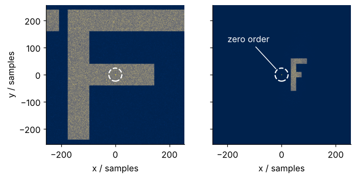
Two focal-plane images of 512 by 512 samples after a 64-sample shift, a dashed circle marking the zero order at the center. Left: an F filling the window; its right end wraps around to the left edge. Right: the bordered F, moved to the right and intact.

The fix is to keep the target within the central half of the window, as Step 1 did.

Stagnation. Symptom: the error flattens after a dozen rounds, and more rounds change nothing. Cause: GS only ever moves downhill in \(\varepsilon\), so it stops in the nearest local minimum, and the start phase decides which one. Eight start phases, each from its own generator spawned from rng:

results = []
for child in rng.spawn(8):
    phi, _, eff = gerchberg_saxton(A, T_spots, child.uniform(0, 2 * np.pi, A.shape), 50)
    results.append((uniformity(focal_intensity(A, phi)[on]), eff[-1]))
u_all, eta_all = np.array(results).T
print(f"uniformity from {u_all.min():.3f} to {u_all.max():.3f}, efficiency from {eta_all.min():.3f} to {eta_all.max():.3f}")

uniformity from 0.485 to 0.747, efficiency from 0.606 to 0.618

The efficiency hardly depends on the start, but the uniformity does, by a factor of 1.5 between the worst and the best start. Run a few restarts and keep the best; for spot arrays, the weighted variant below removes the unequal spots directly.

Variations

Weighted GS for equal spots (Di Leonardo and coworkers). In the loop, multiply T at each spot by a weight before it replaces the amplitude of F, and update the weights every round as weights *= np.mean(np.abs(F[on])) / np.abs(F[on]), so a weak spot asks for more light next time.
A phase from two measured intensities. This is the problem Gerchberg and Saxton solved. Replace A and T by the square roots of the two measured intensities, each background-subtracted and on the same pixel grid; the loop is unchanged, and the returned phi is the phase in the first plane.
Hybrid input-output (Fienup). For a single measured diffraction pattern, T is the square root of its intensity, and the field g in the first plane is known only to be zero outside a region, its support. In the loop, replace the line that computes phi by g_new = to_slm(T * np.exp(1j * np.angle(F))) and g = np.where(support, g_new, g - beta * g_new), with g starting as the first guess and beta a constant such as 0.9, then transform g instead of A * np.exp(1j * phi). Setting g to zero outside the support instead would be Fienup's error reduction, GS with a support; the feedback from the previous g pushes the iteration out of stagnation.
Three-dimensional patterns. A quadratic phase -np.pi * r**2 / (wavelength * f_lens) acts as a lens and moves a spot above or below the focal plane; propagate between planes with the angular spectrum method.

Cheat sheet

to_focal = lambda E: np.fft.fftshift(np.fft.fft2(np.fft.ifftshift(E), norm="ortho"))
to_slm = lambda F: np.fft.fftshift(np.fft.ifft2(np.fft.ifftshift(F), norm="ortho"))
F = to_focal(A * np.exp(1j * phi))                       # A, T: beam and target amplitudes, equal power
phi = np.angle(to_slm(T * np.exp(1j * np.angle(F))))     # one GS round; repeat these two lines
err = np.sqrt(np.sum((np.abs(F) - T)**2) / np.sum(T**2)) # never rises
I_t = np.abs(F[T > 0])**2                                # intensity on the target samples
eta = I_t.sum() / np.sum(np.abs(F)**2)                   # diffraction efficiency
u = 1 - (I_t.max() - I_t.min()) / (I_t.max() + I_t.min())                       # uniformity of the spots
phi_q = np.round(np.mod(phi, 2*np.pi) / (2*np.pi) * 256) % 256 * (2*np.pi / 256) # 8 bits
phi_g = np.mod(phi + 2*np.pi * 64 * np.arange(N) / N, 2*np.pi)                   # 64 samples off the zero order