Steady heat conduction with scikit-fem: a steel plate with a hole (Python)

The problem: how much heat gets past a hole?

Clamp a square plate of carbon steel between a hot block and a cold one: L = 0.1 m on a side, conductivity k = 50 W/(m K), the left edge at 80 °C, the right edge at 20 °C, the top and the bottom insulated. Without a hole, steady heat conduction through it is one line of arithmetic: the plate is as tall as it is long, so Q₀ = k ΔT = 3000 W per meter of thickness gets through. Now drill a bolt hole of radius a = 0.015 m through the middle, insulated like the free edges, and the heat has to go around it. How much of Q₀ still gets through, and where is the temperature gradient steepest?

The temperature obeys the steady heat equation without a source,

\[-\nabla\cdot(k\,\nabla T) = 0 ,\]

which for constant k is the Poisson equation of scikit-fem from the ground up: the sag of a membrane under pressure with zero load and T in place of u. None of scikit-fem's built-in meshes has a hole, so the mesh comes from Gmsh, and two edges are held at temperatures other than zero while three are left free. The hole takes φ = πa²/L² = 7.07 % of the plate's area, and both answers turn out to depend on that fraction.

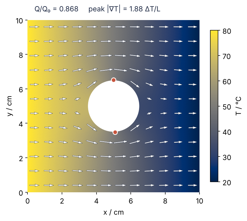
Temperature over the steel plate in °C, x and y in cm, from 80 at the left edge to 20 at the right. White arrows of heat flow bend around the central hole; two dots at the top and the bottom of the hole mark the gradient peak, 1.88 times ΔT/L. Q/Q₀ = 0.868.

This is where we end up: the temperature in the cividis colormap, the heat flow bending around the hole, and dots where the gradient peaks. 86.8 % of Q₀ gets through. Step 6 draws it from a mesh of 86,417 triangles.

Setup

Install both packages with pip install scikit-fem gmsh. On Linux the gmsh wheel needs X11, OpenGL, and OpenMP libraries that a minimal system lacks, and on Debian and Ubuntu one line installs them: apt-get install libglu1-mesa libgl1 libxft2 libxcursor1 libxinerama1 libgomp1.

import numpy as np
import matplotlib.pyplot as plt
import matplotlib.tri as mtri
import gmsh
from skfem import MeshTri, Basis, ElementTriP1, BilinearForm, asm, condense, solve
from skfem.helpers import dot, grad

L, A_HOLE, K = 0.1, 0.015, 50.0       # m, m, W/(m K); A_HOLE so that A stays free for the matrix
T_HOT, T_COLD = 80.0, 20.0            # °C
Q0 = K * (T_HOT - T_COLD)             # W per m of thickness, plate without the hole
G0 = (T_HOT - T_COLD) / L             # K/m, the applied gradient
PHI = np.pi * A_HOLE**2 / L**2        # area fraction of the hole
RAYLEIGH = (1 - PHI) / (1 + PHI)      # Q/Q0 for a square array of insulating cylinders, Step 6's reference

plt.rcParams.update({
    "figure.figsize": (7, 3.6), "figure.dpi": 110,
    "axes.spines.top": False, "axes.spines.right": False,
    "axes.grid": True, "grid.alpha": 0.25,
    "font.size": 11, "lines.linewidth": 1.8,
})
INK, ACCENT, SECOND, MUTED = "#1f2a44", "#c8553d", "#2a7f9e", "#8a8f98"

print(f"Q0 = {Q0:.0f} W/m, nominal gradient {G0:.0f} K/m, phi = {PHI:.4f}, Rayleigh Q/Q0 = {RAYLEIGH:.5f}")

Q0 = 3000 W/m, nominal gradient 600 K/m, phi = 0.0707, Rayleigh Q/Q0 = 0.86796

Step 1: Draw the plate with a hole in Gmsh and hand it to MeshTri

Gmsh builds a geometry the way you would sketch the part: a rectangle, a disk, the disk cut out. The sketching happens in gmsh.model.occ, the OpenCASCADE geometry kernel, which keeps its shapes apart from the model the mesher reads. addRectangle (a corner, then width and height) and addDisk (a center, then two radii) return integer tags, and cut subtracts one list of shapes from another, each named by a (dimension, tag) pair: (2, plate) is a surface. synchronize copies the shapes into the model; forget it and the mesher finds nothing. Mesh.MeshSizeMax is the longest element edge h, mesh.generate(2) meshes the surfaces, and General.Terminal 0, set first, keeps Gmsh's log out of the cell. Mesh.MeshSizeFromCurvature waits for the second pitfall.

getNodes returns node tags and the coordinates flat, x, y, z for each node in turn. getElementsByType(2) returns the node tags of the three-node triangles, Gmsh's element type 2, also flat, and a reshape makes it three per triangle. Tags count from 1 and may have gaps, so a lookup array index[tags] = arange(n) turns them into the column numbers MeshTri expects. gmsh.finalize frees the model.

def plate_mesh(h, per_turn=0):
    gmsh.initialize()
    gmsh.option.setNumber("General.Terminal", 0)
    occ = gmsh.model.occ
    plate = occ.addRectangle(0, 0, 0, L, L)
    hole = occ.addDisk(L / 2, L / 2, 0, A_HOLE, A_HOLE)
    occ.cut([(2, plate)], [(2, hole)])
    occ.synchronize()
    gmsh.option.setNumber("Mesh.MeshSizeMax", h)
    gmsh.option.setNumber("Mesh.MeshSizeFromCurvature", per_turn)   # 0 is off; see Pitfalls
    gmsh.model.mesh.generate(2)
    tags, xyz, _ = gmsh.model.mesh.getNodes()
    _, tri_tags = gmsh.model.mesh.getElementsByType(2)
    gmsh.finalize()
    index = np.zeros(tags.max() + 1, dtype=np.int64)
    index[tags] = np.arange(len(tags))
    p = xyz.reshape(-1, 3)[:, :2].T                 # drop z: 2 x N
    t = index[tri_tags].reshape(-1, 3).T            # 3 x M
    return MeshTri(np.ascontiguousarray(p), np.ascontiguousarray(t))   # else skfem warns it changes the memory layout

def on_circle(mesh):
    return np.isclose(np.hypot(mesh.p[0] - L / 2, mesh.p[1] - L / 2), A_HOLE)

mesh = plate_mesh(2e-3)
print(mesh)
print(f"boundary nodes: {len(mesh.boundary_nodes())}, on the hole: {on_circle(mesh).sum()}")

<skfem MeshTri1 object>
  Number of elements: 5544
  Number of vertices: 2896
  Number of nodes: 2896
boundary nodes: 248, on the hole: 48

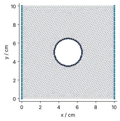
2,896 nodes and 5,544 triangles at h = 2 mm. The circle carries 48 of the 248 boundary nodes, so the hole the solver sees is a polygon of 48 sides with its corners on the circle:

Show code

held = np.isclose(mesh.p[0], 0) | np.isclose(mesh.p[0], L)
fig, ax = plt.subplots(figsize=(4, 4))
ax.triplot(100 * mesh.p[0], 100 * mesh.p[1], mesh.t.T, color=MUTED, lw=0.4)
ax.plot(100 * mesh.p[0, held], 100 * mesh.p[1, held], "o", color=SECOND, ms=3)
ax.plot(100 * mesh.p[0, on_circle(mesh)], 100 * mesh.p[1, on_circle(mesh)], "o", color=INK, ms=3)
ax.set(xlabel="x / cm", ylabel="y / cm", aspect="equal", xlim=(-0.3, 10.3), ylim=(-0.3, 10.3))
ax.grid(False)
plt.show()

The 2 mm mesh of the plate in gray, 5,544 triangles, x and y in cm from 0 to 10. The hole is a polygon whose 48 corners, marked as dark dots, sit on the circle; the nodes of the held left and right edges are marked in blue.

Step 2: Hold two edges at 80 and 20 °C with condense

The assembly is the membrane's stiffness form with no load, and the form leaves k out: k would scale A and the zero right-hand side alike, so T does not depend on it. Step 4 puts it back into the flux.

The membrane was clamped at zero; here the left edge is held at 80 °C and the right at 20 °C. Split the columns of A into free nodes I and held nodes D. The row of a free node then reads \(A_{II} T_I + A_{ID} T_D = 0\), and the held temperatures in it are known, so their part moves to the right:

\[A_{II}\, T_I = -A_{ID}\, T_D .\]

condense(A, b, x=T0, D=fixed) does that with the values in T0: it drops the rows of the held nodes and moves their columns to the right, and solve writes 80 and 20 back. Finite elements: hat functions, the weak form, and a heated bar describes the same move for a bar.

@BilinearForm
def conduction(u, v, w):
    return dot(grad(u), grad(v))

basis = Basis(mesh, ElementTriP1())
A = asm(conduction, basis)
left = np.flatnonzero(np.isclose(mesh.p[0], 0))
right = np.flatnonzero(np.isclose(mesh.p[0], L))
fixed = np.concatenate([left, right])
T0 = np.zeros(mesh.p.shape[1])
T0[left], T0[right] = T_HOT, T_COLD

Ac, bc, Tc, I = condense(A, np.zeros_like(T0), x=T0, D=fixed)
print(f"unknowns: {Ac.shape[0]}, nonzero right-hand side entries: {np.count_nonzero(bc)}")
T = solve(Ac, bc, Tc, I)

top = np.argmin(np.hypot(mesh.p[0] - L / 2, mesh.p[1] - (L / 2 + A_HOLE)))
bottom = np.argmin(np.hypot(mesh.p[0] - L / 2, mesh.p[1] - (L / 2 - A_HOLE)))
print(f"T from {T.min():.1f} to {T.max():.1f} °C; top of the hole {T[top]:.4f} °C, bottom {T[bottom]:.4f} °C")

unknowns: 2794, nonzero right-hand side entries: 105
T from 20.0 to 80.0 °C; top of the hole 50.0008 °C, bottom 49.9967 °C

2,794 unknowns: 2,896 nodes less 51 on each held edge. The right-hand side has 105 nonzero entries, one per free node sharing a triangle with a held one: the moved columns, made visible. T stays between 20 and 80 °C and is 50.00 °C at the top and the bottom of the hole, the mid-temperature, because the plate is antisymmetric about x = L/2. The mesh is not quite, hence the thousandths.

Step 3: Leave the other edges alone: that is the insulation

Step 2 never mentions the top, the bottom, or the hole. Their nodes stay free, and that alone insulates them. The edge term of the membrane tutorial's Step 2, \(\oint v\,\partial T/\partial n\,ds\), vanished there because v was zero on the clamped edges. Here the hat functions of the free boundary nodes are not zero on their edges, yet the weak form \(\int \nabla T\cdot\nabla v\,dA = 0\) must hold for every one of them. Integrated by parts, its left side is the heat equation inside, which holds, plus that edge term, so the edge term must vanish for every such v. That forces \(\partial T/\partial n = 0\) along those edges: no heat crosses. Writing nothing imposes zero flux, a natural boundary condition, enforced by the weak form instead of node by node.

Enforced weakly, it holds exactly only in the limit. Wrap Step 2 in a function and measure, on triangles with an edge on the hole, the slope across it as a fraction of the gradient:

def temperature(mesh):
    basis = Basis(mesh, ElementTriP1())
    A = asm(conduction, basis)
    left = np.flatnonzero(np.isclose(mesh.p[0], 0))
    right = np.flatnonzero(np.isclose(mesh.p[0], L))
    T0 = np.zeros(mesh.p.shape[1])
    T0[left], T0[right] = T_HOT, T_COLD
    T = solve(*condense(A, np.zeros_like(T0), x=T0, D=np.concatenate([left, right])))
    return basis, A, T, left, right

boundary = mesh.boundary_nodes()
print(f"boundary nodes: {len(boundary)}, held: {len(fixed)}, free: {len(np.setdiff1d(boundary, fixed))}")
for h in [2e-3, 1e-3]:
    mesh_h = plate_mesh(h)
    basis_h, _, T_h, _, _ = temperature(mesh_h)
    at_hole = on_circle(mesh_h)[mesh_h.t].sum(axis=0) == 2       # triangles with an edge on the circle
    g = basis_h.interpolate(T_h).grad[:, :, 0][:, at_hole]
    n = mesh_h.p[:, mesh_h.t[:, at_hole]].mean(axis=1) - L / 2   # from the center to the centroid
    n /= np.linalg.norm(n, axis=0)
    print(f"h = {h * 1e3:.0f} mm: median |dT/dn| / |grad T| on the hole = {np.median(np.abs((g * n).sum(axis=0)) / np.linalg.norm(g, axis=0)):.3f}")

boundary nodes: 248, held: 102, free: 146
h = 2 mm: median |dT/dn| / |grad T| on the hole = 0.079
h = 1 mm: median |dT/dn| / |grad T| on the hole = 0.040

Of 248 boundary nodes, 146 are left free. The slope across the hole is 7.9 % of the gradient at 2 mm and 4.0 % at 1 mm, in the median: it halves with h, the first-order slope accuracy of the membrane tutorial's Step 4.

Step 4: Read the heat flux off the rows of A @ T

The heat crosses the held edges, and the matrix already holds it. Row i of A @ T is \(\int \nabla\varphi_i\cdot\nabla T\,dA\). For the exact temperature, the integration by parts of Step 3 turns it into

\[(A T)_i = \oint \varphi_i\,\frac{\partial T}{\partial n}\,ds ,\]

the slope across the boundary, weighted by node i's hat function. For a free node, inside or on an insulated edge, the row is an equation solve satisfied with zero on the right, so it is zero to rounding. The held nodes' rows were dropped in Step 2, and nothing forced them to zero. By Fourier's law q = −k∇T the inflow is \(k\,\partial T/\partial n\) with the outward normal, so k times such a row is the heat the block feeds through node i's share of the edge. Summed,

\[Q_\text{in} = k \sum_\text{left} (A T)_i , \qquad Q_\text{out} = -k \sum_\text{right} (A T)_i ,\]

with the minus because heat leaves on the right. With lengths in meters, A is dimensionless in two dimensions and both sums are in W/m.

The two must agree. The rows of A sum to zero (the first pitfall of the membrane tutorial) and A is symmetric, so the entries of \(AT\) add up to \(\mathbf 1^\mathsf{T} A T = (A\mathbf 1)^\mathsf{T} T = 0\). The free rows are zero, so the left sum is minus the right sum: the plate's heat balance, exact on any mesh.

R = A @ T
Q_in, Q_out = K * R[left].sum(), -K * R[right].sum()
free = np.setdiff1d(np.arange(len(T)), fixed)
print(f"Q_in = {Q_in:.2f} W/m, Q_out = {Q_out:.2f} W/m, largest free row {np.abs(R[free]).max():.1e}")
print(f"Q/Q0 = {Q_in / Q0:.5f}")

Q_in = 2606.02 W/m, Q_out = 2606.02 W/m, largest free row 1.8e-13
Q/Q0 = 0.86867

2606.02 W/m in and the same out, the free rows at 1.8e-13. Q/Q₀ = 0.8687 on this mesh: a 1 cm thick plate passes 26.1 W instead of 30 W.

Step 5: Find where the gradient peaks

basis.interpolate(T).grad[:, :, 0] gives the gradient per triangle, as in the membrane tutorial's Step 5. The peak comes as a mirror pair, so take the largest |∇T| in the lower and the upper half of the plate, by triangle centroid:

slope = np.linalg.norm(basis.interpolate(T).grad[:, :, 0], axis=0)
centroid = mesh.p[:, mesh.t].mean(axis=1)
for name, half in [("lower", centroid[1] < L / 2), ("upper", centroid[1] > L / 2)]:
    j = np.flatnonzero(half)[np.argmax(slope[half])]
    print(f"{name} half: peak {slope[j] / G0:.3f} x dT/L at ({100 * centroid[0, j]:.2f}, {100 * centroid[1, j]:.2f}) cm")
print(f"2/(1 + phi) = {2 / (1 + PHI):.3f}")

lower half: peak 1.875 x dT/L at (4.91, 3.46) cm
upper half: peak 1.868 x dT/L at (4.89, 6.55) cm
2/(1 + phi) = 1.868

1.875 and 1.868 times the applied 600 K/m, at the bottom and the top of the hole. On the insulated hole the gradient is all tangential, and the heat crowds past where the path is narrowest.

For an isolated hole in a uniform gradient the peak is exactly 2, from potential flow around a cylinder. This plate stays below because its edges act as mirrors. Reflect the plate with its hole and its temperature field across an insulated edge, and T continues unchanged, since no heat crosses there, as none crosses a symmetry plane. Reflect it across a held edge and flip the sign of T minus the edge value, and the gradient runs on unbroken into the copy. So the plate is one cell of an endless square array of holes in a uniform gradient, each shielded by its neighbors up- and downstream. The theory of such arrays (Rayleigh, Maxwell Garnett) puts the gradient a hole feels, to first order, at the applied one divided by 1 + φ. Take that as a quoted result; the mirrors alone do not give it. It predicts 2/(1 + φ) = 1.868, within half a percent of the computed peaks, and it tends to 2 as the plate grows around the same hole. The gradient is not the thermal stress, which needs an elasticity solve.

Step 6: Refine against Rayleigh's value and draw the plate

The mirrors of Step 5 also give a reference for the flux. Q/Q₀ is the array's effective conductivity, the conductivity a plate without holes would need to pass the same heat, divided by k. Rayleigh found it to be (1 − φ)/(1 + φ), with corrections of order φ⁵. Wrap Steps 2, 4, and 5 in a function and run it on four meshes:

def solve_plate(mesh):
    basis, A, T, left, right = temperature(mesh)
    R = A @ T
    slope = np.linalg.norm(basis.interpolate(T).grad[:, :, 0], axis=0)
    return T, K * R[left].sum(), -K * R[right].sum(), slope

print("h / mm  triangles    Q/Q0     error   ratio   peak / G0")
err_prev = None
for h in [4e-3, 2e-3, 1e-3, 5e-4]:
    mesh_h = plate_mesh(h)
    T_h, Q_in_h, Q_out_h, slope_h = solve_plate(mesh_h)
    err = Q_in_h / Q0 - RAYLEIGH
    ratio = f"{err_prev / err:5.2f}" if err_prev else "     "
    print(f"{1e3 * h:6.1f}  {mesh_h.t.shape[1]:9,d}  {Q_in_h / Q0:.5f}  {err:.2e}  {ratio}   {slope_h.max() / G0:.3f}")
    err_prev = err
print(f"Rayleigh {RAYLEIGH:.5f}, phi^5 = {PHI**5:.1e}")
print(f"2 mm mesh of Step 4: Q_in = {Q_in:.2f} W/m, k T.AT / dT = {K * T @ R / (T_HOT - T_COLD):.2f} W/m")

h / mm  triangles    Q/Q0     error   ratio   peak / G0
   4.0      1,430  0.87076  2.80e-03          1.868
   2.0      5,544  0.86867  7.13e-04   3.92   1.875
   1.0     21,773  0.86814  1.80e-04   3.96   1.875
   0.5     86,417  0.86801  4.45e-05   4.05   1.878
Rayleigh 0.86796, phi^5 = 1.8e-06
2 mm mesh of Step 4: Q_in = 2606.02 W/m, k T.AT / dT = 2606.02 W/m

The error falls by 3.92, 3.96, and 4.05 per halving, as h², and on 86,417 triangles Q/Q₀ = 0.86801 against Rayleigh's 0.86796. That is faster than the slopes the flux is made of, and the last line says why. With the free rows zero and the edges at 80 and 20 °C, Step 4's sums add up to \(k\,T^\mathsf{T}AT/\Delta T\), the integral of \(k|\nabla T|^2/\Delta T\) over the plate. An energy like that misses by the square of the slope error, h times h, which is why the flux is read off the rows and not off the slopes. The remaining 4.45e-5 is about 25 times φ⁵, so it belongs to the mesh and not to Rayleigh's truncation. The gradient peak reads 1.868, 1.875, 1.875, 1.878: a per-triangle slope converges only as h, and the third digit is still moving. Quote it as 1.88.

centroid_h = mesh_h.p[:, mesh_h.t].mean(axis=1)                    # the last pass of the loop: 0.5 mm
peaks = [np.flatnonzero(half)[np.argmax(slope_h[half])]
         for half in (centroid_h[1] < L / 2, centroid_h[1] > L / 2)]
tri = mtri.Triangulation(100 * mesh_h.p[0], 100 * mesh_h.p[1], mesh_h.t.T)   # in cm
gx, gy = np.meshgrid(np.linspace(0.4, 9.6, 12), np.linspace(0.4, 9.6, 12))
dTdx, dTdy = mtri.LinearTriInterpolator(tri, T_h).gradient(gx, gy)          # masked inside the hole
qx, qy = -K * 100 * dTdx, -K * 100 * dTdy                                    # W/m², from K/cm

fig, ax = plt.subplots(figsize=(6, 5))
field = ax.tripcolor(tri, T_h, cmap="cividis", shading="gouraud")
ax.quiver(gx, gy, qx, qy, color="white", scale_units="xy", scale=5e4, width=0.005,
          edgecolor=INK, linewidth=0.3, pivot="mid")                  # centered on the grid points
ax.plot(*(100 * centroid_h[:, peaks]), "o", color=ACCENT, ms=7, mec="white", mew=1.2)
ax.text(0.4, 10.4, f"Q/Q₀ = {Q_in_h / Q0:.3f}     peak |∇T| = {slope_h.max() / G0:.2f} ΔT/L",
        color=INK, va="bottom")
ax.set(xlabel="x / cm", ylabel="y / cm", aspect="equal", xlim=(0, 10), ylim=(0, 10))
ax.spines[["left", "bottom"]].set_visible(False)
ax.grid(False)
fig.colorbar(field, ax=ax, label="T / °C", shrink=0.85)
plt.show()

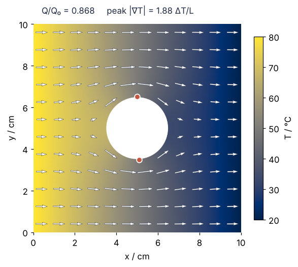
Temperature over the steel plate in °C, x and y in cm, from 80 at the left edge to 20 at the right. White arrows of heat flow bend around the central hole; two dots at the top and the bottom of the hole mark the gradient peak, 1.88 times ΔT/L. Q/Q₀ = 0.868.

Without the hole every arrow would point right with the same length, a flux of k ΔT/L = 30 kW/m². With it, the arrows in front of and behind the hole shrink to almost nothing, and the longest pass beside the two dots, where the flux reaches 1.88 times that.

Pitfalls

Clamping every boundary node out of habit. The membrane tutorial passed D=mesh.boundary_nodes(), and the hand does it again. Here that also holds the top, the bottom, and the hole, at whatever T0 contains there, which is zero:

T_all = solve(*condense(A, np.zeros_like(T0), x=T0, D=mesh.boundary_nodes()))
R_all = A @ T_all
print(f"all boundary nodes held: Q_in = {K * R_all[left].sum():,.0f} W/m, Q_out = {-K * R_all[right].sum():,.0f} W/m")

all boundary nodes held: Q_in = 24,404 W/m, Q_out = -6,048 W/m

Heat now enters at both ends and drains into a hole held at 0 °C, so Q_out is negative and more than nine times as much enters on the left as with the right D. The fix is to put into D only the edges whose temperature you know. The balance check of Step 4 catches this at once, which is the reason to print both sums every time.

A hole drawn with too few points. On a coarse mesh Q/Q₀ comes out high, at 4 mm by 2.8e-3. Part of the cause is the polygon: its corners sit on the circle, so it is slightly smaller than the true hole and lets more heat past. Mesh.MeshSizeFromCurvature set to N asks Gmsh for N elements per full turn of a curve, and keeps the rest of the plate coarse:

for per_turn in [0, 80]:
    mesh_c = plate_mesh(4e-3, per_turn)
    _, Q_in_c, _, _ = solve_plate(mesh_c)
    print(f"h = 4 mm, {per_turn:2d} per turn: {on_circle(mesh_c).sum():2d} nodes on the hole, "
          f"{mesh_c.t.shape[1]:,d} triangles, Q/Q0 = {Q_in_c / Q0:.5f}")

h = 4 mm,  0 per turn: 24 nodes on the hole, 1,430 triangles, Q/Q0 = 0.87076
h = 4 mm, 80 per turn: 80 nodes on the hole, 3,176 triangles, Q/Q0 = 0.86834

80 elements per turn instead of 24 bring the error from 2.8e-3 to 3.8e-4 on 3,176 triangles, better than the uniform 2 mm mesh of Step 6 with 5,544. Curved boundaries deserve the refinement; the open plate does not.

Gmsh's model outlives your function. Gmsh keeps one global model. Mesh twice without gmsh.finalize() or gmsh.clear() in between and the second call adds a second rectangle and a second disk to the first, so the triangle count doubles and no longer follows h. Without General.Terminal 0 the cell fills with Gmsh's log, which carries timings, so two runs of the notebook no longer give the same output. Initialize, set the terminal option, and finalize inside the mesh function, as plate_mesh does.

Variations

Another outline. A polygon from occ.addPoint at each corner, occ.addLine between them, occ.addCurveLoop, and occ.addPlaneSurface, then the same cut; a rectangle with filleted corners from occ.addRectangle(..., roundedRadius=r); or a part straight from CAD with gmsh.open("part.step"). The rest of plate_mesh stays, and only the masks for the held edges change.
A second hole. One more occ.addDisk in the tool list of cut, [(2, hole1), (2, hole2)]. Two holes stacked across the flow push the peak gradient up; two in a row along the flow lower it, by the shielding of Step 5.
Edges by name instead of by coordinate. gmsh.model.addPhysicalGroup(1, curve_tags, name="hot") before meshing, then gmsh.model.mesh.getNodesForPhysicalGroup(1, tag) returns that edge's nodes. This finds the held nodes on an outline where np.isclose(x, 0) no longer works.
A convective edge. Replace an insulated edge with heat transfer to air at a coefficient h_c in W/(m² K). FacetBasis(mesh, ElementTriP1(), facets=...) is a basis whose integrals run along the chosen boundary edges instead of over the triangles; a BilinearForm with \(h_c\,u\,v/k\) and a LinearForm with \(h_c\,T_\infty\,v/k\) on it, divided by k because Step 2 left k out of A, add to A and to the right-hand side. The edge term of Step 3 no longer vanishes; it becomes \(-h_c (T - T_\infty)/k\), a Robin condition.

Cheat sheet

occ = gmsh.model.occ                                    # after gmsh.initialize(); General.Terminal 0
occ.cut([(2, occ.addRectangle(0, 0, 0, L, L))], [(2, occ.addDisk(xc, yc, 0, a, a))])
occ.synchronize()                                       # hand the shapes to the mesher
gmsh.option.setNumber("Mesh.MeshSizeMax", h); gmsh.model.mesh.generate(2)
index[tags] = np.arange(len(tags))                      # Gmsh tags -> MeshTri columns, then gmsh.finalize()
mesh = MeshTri(xyz.reshape(-1, 3)[:, :2].T, index[tri_tags].reshape(-1, 3).T)
T = solve(*condense(A, 0 * T0, x=T0, D=fixed))          # known columns move to the right
                                                        # insulated edges: leave them out of D, write nothing
Q_in = k * (A @ T)[left].sum()                          # W/m; must equal -k * (A @ T)[right].sum()
slope = np.linalg.norm(basis.interpolate(T).grad[:, :, 0], axis=0)   # |grad T| per triangle