Finite elements: hat functions, the weak form, and a heated bar
Afterwards you can say what a finite element solution is, build a 1D stiffness matrix from the weak form, and tell how the error falls with element size.
- Topic
- Finite elements
- Field
- Engineering, Mathematics, Physics
- Prerequisites
- none beyond Python basics
- Libraries
matplotlib 3.11.2numpy 2.4.3skfem 12.0.2
py-finite-elements.ipynb, executed with the versions above. The download needs a free account
Run it yourself. In a terminal, this installs exactly the versions above:
pip install numpy==2.4.3 skfem==12.0.2 matplotlib==3.11.2 jupyterlabThe question
A wire that carries a current heats itself evenly along its length, q watts per cubic meter, and its two ends are clamped to blocks at the temperature of the room. With conductivity k, the excess temperature u(x) of a bar of length L obeys \(-k\,u'' = q\) with \(u(0) = u(L) = 0\), and the answer is a parabola, \(u = q\,x(L - x)/(2k)\), with its peak \(qL^2/(8k)\) in the middle. Measure x in units of L and u in units of \(qL^2/k\), and every such bar becomes the same bar, with a peak of 0.125. Here it is next to its finite element solution with four elements:
Show code
import numpy as np
import matplotlib.pyplot as plt

plt.rcParams.update({
    "figure.figsize": (8, 3.2), "figure.dpi": 110,
    "axes.spines.top": False, "axes.spines.right": False,
    "axes.grid": True, "grid.alpha": 0.25,
    "font.size": 11, "lines.linewidth": 1.8,
})
INK, ACCENT, SECOND, MUTED = "#1f2a44", "#c8553d", "#2a7f9e", "#8a8f98"

L, q, k = 1.0, 1.0, 1.0                     # u in units of qL²/k, x in units of L
x = np.linspace(0, L, 4001)

def exact(x):
    return q * x * (L - x) / (2 * k)

def fem_bar(n):
    """Nodes and nodal temperatures of the n-element solution (assembled step by step under Formalization)."""
    h = L / n
    K = k / h * (2 * np.eye(n - 1) - np.eye(n - 1, k=1) - np.eye(n - 1, k=-1))
    U = np.linalg.solve(K, np.full(n - 1, q * h))
    return np.linspace(0, L, n + 1), np.r_[0, U, 0]

nodes4, U4 = fem_bar(4)
x_mid = 0.125                                # midpoint of the first element, where the gap is largest
fig, ax = plt.subplots()
ax.plot(x, exact(x), color=INK)
ax.plot(nodes4, U4, "o-", color=ACCENT, ms=6)
gap = exact(x_mid) - np.interp(x_mid, nodes4, U4)
ax.annotate(f"largest gap {gap:.4f}", xy=(x_mid, exact(x_mid) - gap / 2), xytext=(0.17, 0.018),
            color=MUTED, arrowprops=dict(arrowstyle="-", color=MUTED, lw=1))
ax.text(0.5, exact(0.5) + 0.006, f"peak {exact(0.5):.3f}", ha="center")
ax.text(0.13, 0.095, "exact", color=INK, ha="right")              # direct labels instead of a legend
ax.text(0.83, 0.043, "4 elements", color=ACCENT, ha="right")
ax.set(xlabel="x / L", ylabel="u / (qL²/k)", xlim=(0, 1), ylim=(0, 0.145))
plt.show()
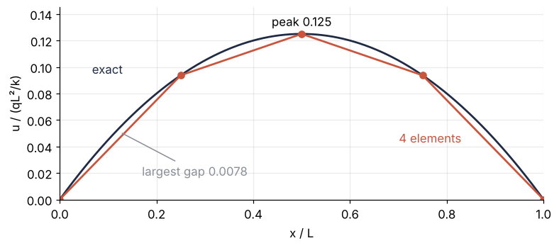
Some of it is obvious. The finite element solution is five points joined by straight lines, the points sit on the parabola, and the straight pieces cut below the arch, by at most 0.0078 at the middle of each element, against a peak of 0.125.
What is not obvious is how the points were found. The method never asked for the temperature at a point. It asked for the best combination of tent-shaped functions, one per node, and it asks the same question on a mesh of triangles fitted to any outline, a disk or a turbine blade, where a method built on point values lays its points in rows and columns and has to patch every place where a curved edge cuts between them. So three questions. What is the combination, what makes it "best", and why do the nodes come out exact when nothing aimed at them?
The idea: build the temperature from hats
Put a node at each end of every element: with four elements on the bar, that is five nodes, three of them inside. Over each interior node j stands a hat \(\varphi_j\), a tent that is 1 at node j, 0 at every other node, and straight in between. Add the hats with weights, \(u_h = \sum_j U_j \varphi_j\), and you get a broken line. At node j only hat j is nonzero, and there it is 1, so the broken line passes through the point \((x_j, U_j)\).
The weight is the temperature at the node. Choosing a solution means choosing three numbers.
Show code
def hat(j, nodes, x):
    """Hat function of node j: 1 at that node, 0 at all others, linear in between."""
    return np.interp(x, nodes, np.eye(nodes.size)[j])

U_guess = np.array([0, 0.05, 0.15, 0.05, 0])   # an arbitrary choice, for comparison

fig, axes = plt.subplots(3, 1, figsize=(8, 6.3), sharex=True)
for j in (1, 2, 3):
    axes[0].plot(x, hat(j, nodes4, x), color=MUTED, lw=1.2)
axes[0].set(ylabel="hat", ylim=(0, 1.1))
for ax, U, color in ((axes[1], U_guess, SECOND), (axes[2], U4, ACCENT)):
    ax.plot(x, exact(x), color=INK)
    if ax is axes[2]:
        for j in (1, 2, 3):
            ax.plot(x, U[j] * hat(j, nodes4, x), color=ACCENT, lw=1.0)
    ax.plot(nodes4, U, "o-", color=color, ms=6)
    for xj, Uj in zip(nodes4[1:-1], U[1:-1]):
        ax.text(xj, Uj + 0.012, f"{Uj:.3f}", ha="center", color=color)
    ax.set(ylabel="u / (qL²/k)", ylim=(0, 0.175))
axes[-1].set(xlabel="x / L", xlim=(0, 1))
plt.show()
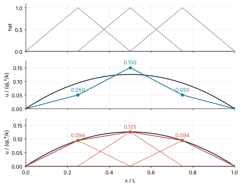
The top panel shows the three hats. In the middle, weights 0.05, 0.15, and 0.05 give a broken line that is nowhere near the parabola: a legitimate member of the family, and a bad one. In the bottom panel the finite element weights, 0.094, 0.125, and 0.094, scale each hat to its node's height (the thin lines), and their sum runs through the parabola at every node.
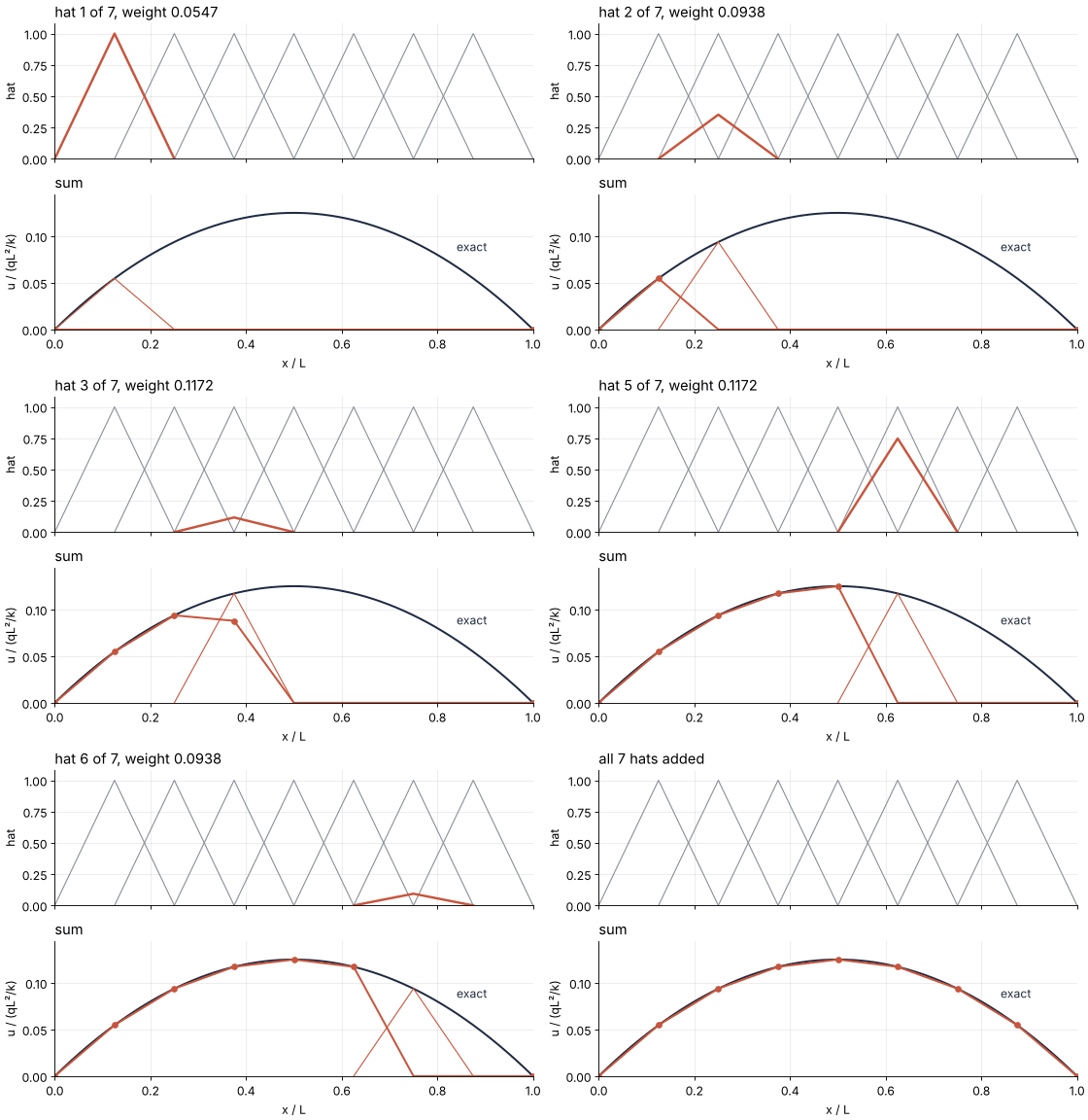
With more elements the family grows and the broken line hugs the curve more closely. On eight elements there are seven hats, and the sum builds up one weighted hat at a time:
Show code
"""Hat sum: a finite element solution built one weighted hat function at a time.

Renders ../../assets/hat-sum.gif for the heated bar of py-finite-elements, eight elements.
Run it from any directory:

    python scene.py
"""
from pathlib import Path

import numpy as np
import matplotlib.pyplot as plt
from matplotlib.animation import FuncAnimation, PillowWriter
from PIL import Image

OUT = Path(__file__).resolve().parents[2] / "assets" / "hat-sum.gif"
INK, ACCENT, SECOND, MUTED = "#1f2a44", "#c8553d", "#2a7f9e", "#8a8f98"
plt.rcParams.update({"axes.spines.top": False, "axes.spines.right": False,
                     "axes.grid": True, "grid.alpha": 0.25, "font.size": 11})

# ---- data: the bar in units of qL²/k, eight elements, seven interior nodes
n = 8
h = 1 / n
nodes = np.linspace(0, 1, n + 1)
x = np.linspace(0, 1, 801)
exact = x * (1 - x) / 2
K = (2 * np.eye(n - 1) - np.eye(n - 1, k=1) - np.eye(n - 1, k=-1)) / h
U = np.linalg.solve(K, np.full(n - 1, h))            # the finite element weights, one per interior node

def hat(j):
    """Hat function of interior node j (1 to 7) on its two elements: 1 at its node, 0 at the neighbors."""
    xs = np.linspace(nodes[j - 1], nodes[j + 1], 3)
    return xs, np.array([0.0, 1.0, 0.0])

SHRINK, ADD, HOLD = 8, 4, 16                         # frames per hat: scale to its weight, then add it
frames = [(j, k) for j in range(1, n) for k in range(SHRINK + ADD)] + [(n, 0)] * HOLD

# ---- figure, drawn once
fig, (ax1, ax2) = plt.subplots(2, 1, figsize=(7, 4.8), dpi=80, sharex=True, layout="constrained")
for j in range(1, n):
    ax1.plot(*hat(j), color=MUTED, lw=1.0)
(current,) = ax1.plot([], [], color=ACCENT, lw=2.2)  # the hat being scaled
ax2.plot(x, exact, color=INK, lw=1.8)
(piece,) = ax2.plot([], [], color=ACCENT, lw=1.0)    # the same hat at its weight, on the scale of the sum
(total,) = ax2.plot([], [], color=ACCENT, lw=1.8)
(dots,) = ax2.plot([], [], "o", color=ACCENT, ms=5)
ax1.set(ylabel="hat", ylim=(0, 1.08))
ax2.set(xlabel="x / L", ylabel="u / (qL²/k)", xlim=(0, 1), ylim=(0, 0.145))
title = ax1.set_title("", loc="left")
ax2.set_title("sum", loc="left")
ax2.text(0.84, 0.084, "exact", color=INK)                # direct label above the parabola

# ---- one frame: hat j shrinks from height 1 to its weight, then joins the sum
def update(frame):
    j, k = frame
    done = min(j, n) - 1                            # hats already in the sum
    if j < n:
        xs, ys = hat(j)
        s = min(k / (SHRINK - 1), 1.0)
        current.set_data(xs, (1 + s * (U[j - 1] - 1)) * ys)
        piece.set_data(xs, U[j - 1] * ys)
        title.set_text(f"hat {j} of {n - 1}, weight {U[j - 1]:.4f}")
        if k >= SHRINK:                              # the add phase: the sum grows toward the new hat
            done += (k - SHRINK + 1) / ADD
    else:
        current.set_data([], [])
        piece.set_data([], [])
        title.set_text(f"all {n - 1} hats added")
    weights = np.r_[0, U * np.clip(done - np.arange(n - 1), 0, 1), 0]
    total.set_data(x, np.interp(x, nodes, weights))
    added = np.r_[True, np.arange(n - 1) < done, True]   # dots on the held ends and the hats in the sum
    dots.set_data(nodes[added], weights[added])

# ---- render, and read back what was written
OUT.parent.mkdir(exist_ok=True)
FuncAnimation(fig, update, frames=frames).save(OUT, writer=PillowWriter(fps=12))
plt.close(fig)
with Image.open(OUT) as im:
    delay = im.info["duration"]
    print(f"{OUT.name}: {im.width} x {im.height} px, {im.n_frames} frames at {delay} ms, "
          f"{im.n_frames * delay / 1000:.1f} s, {OUT.stat().st_size / 1024:,.0f} kB")
Every finite element solution is a picture like this one. Elements of higher order use curved pieces instead of straight ones, and in two dimensions the tents stand over triangles, but the solution is always a weighted sum of known shapes, and the method is a rule for the weights.
Testing the equation with each hat
Which weights, then? You cannot demand \(-k\,u'' = q\) point by point of a broken line. Inside each element its second derivative is zero, and at the kinks it is infinite. The finite element method asks for less: multiply the equation by one hat and integrate it along the bar. That turns the equation into a heat balance over the stretch the hat covers, two elements wide, weighted toward its node.
The integral is easier than it looks. The second derivative of a broken line lives only at its kinks: there it is a spike, a Dirac delta, whose area is the jump in slope across the kink. Multiplied by hat \(\varphi_i\), the spike at node i counts with weight 1, and the spikes at the neighboring nodes with weight 0, because that is the value of the hat at each of them. So the integral of \(k\,u_h''\varphi_i\) is k times the slope jump at node i, and the integral of \(q\varphi_i\) is q times the area under the hat, a triangle of base 2h and height 1, which is \(qh\). With the minus sign of the equation, the balance at node i reads
The heat flux is minus k times the slope, counted positive to the right, so the first term is the heat conducted out of node i's patch to the left, the second the heat conducted out to the right, and the right side is the heat generated in it. One balance per hat, so three hats give three equations for the three weights. Here are both sides for the arbitrary weights and for the finite element weights:
Show code
h = L / 4
print("node   arbitrary: out  generated   finite element: out  generated")
for i in (1, 2, 3):
    out_guess = k * (U_guess[i] - U_guess[i - 1]) / h - k * (U_guess[i + 1] - U_guess[i]) / h
    out_fem = k * (U4[i] - U4[i - 1]) / h - k * (U4[i + 1] - U4[i]) / h
    print(f"{i:4d}   {out_guess:15.3f}  {q * h:9.3f}   {out_fem:20.3f}  {q * h:9.3f}")
node   arbitrary: out  generated   finite element: out  generated
   1            -0.200      0.250                  0.250      0.250
   2             0.800      0.250                  0.250      0.250
   3            -0.200      0.250                  0.250      0.250
With the arbitrary weights, node 2 conducts away 0.8 while its patch generates 0.25, and nodes 1 and 3 even take heat in. With the finite element weights, outflow and generation agree at 0.25 in every patch. The balance holds at every node for one set of weights only, and those are the weights.
Formalization
The usual route avoids the spikes and works for curved pieces as well as straight ones. Multiply \(-k\,u'' = q\) by a test function v, a weight like the hat that vanishes at the held ends, \(v(0) = v(L) = 0\). Integrate by parts to move one derivative from u to v. The boundary term \([-k\,u'v]_0^L\) drops out because v is zero at both ends, and what is left is the weak form:
It only asks for first derivatives, which a broken line has. If one end of your bar is insulated instead, the test function no longer has to vanish there: that end keeps its node, and the boundary term drops out anyway, because the flux \(k\,u'\) is zero. Only a held temperature removes a node; if the block is warmer than the room, its known value times its column of K moves to the right side.
Insert \(u = \sum_j U_j\varphi_j\) and \(v = \varphi_i\), one equation per hat, and you get \(KU = f\) with
K is the stiffness matrix and f the load vector. On one element only two hats are nonzero, with slopes \(+1/h\) and \(-1/h\), so each entry is slope times slope times k times the length: \((\pm 1/h)(\pm 1/h)\,k\,h = \pm k/h\). The element matrix is \((k/h)\begin{bmatrix}1 & -1\\ -1 & 1\end{bmatrix}\) and the element load \((qh/2)[1, 1]\), half a hat's area per node. The loop adds them up and drops the rows and columns of the two held end nodes:
n = 4
h = L / n
nodes = np.linspace(0, L, n + 1)
K_all, f_all = np.zeros((n + 1, n + 1)), np.zeros(n + 1)
for e in range(n):                                 # element e joins nodes e and e + 1
    pair = [e, e + 1]
    K_all[np.ix_(pair, pair)] += k / h * np.array([[1, -1], [-1, 1]])   # np.ix_: the 2 x 2 block of the pair
    f_all[pair] += q * h / 2
K, f = K_all[1:-1, 1:-1], f_all[1:-1]              # the ends are held: no unknowns there
U = np.linalg.solve(K, f)

print(f"K =\n{K}\nf = {f}\nU = {U}")
print("U equals the exact nodal values:", np.allclose(U, exact(nodes[1:-1]), rtol=0, atol=1e-15))
tridiag = 2 * np.eye(n - 1) - np.eye(n - 1, k=1) - np.eye(n - 1, k=-1)
print("h K / k equals the [-1, 2, -1] matrix:", np.allclose(h * K / k, tridiag))
K =
[[ 8. -4.  0.]
 [-4.  8. -4.]
 [ 0. -4.  8.]]
f = [0.25 0.25 0.25]
U = [0.09375 0.125   0.09375]
U equals the exact nodal values: True
h K / k equals the [-1, 2, -1] matrix: True
Each row of K is the balance of the previous section, and the solve returns 0.09375, 0.125, and 0.09375.
The same matrix as finite differences, on this mesh. Divide the balance by h and it reads \(k(-U_{i-1} + 2U_i - U_{i+1})/h^2 = q\). The fraction is the change of slope across one spacing divided by the spacing, the approximation of \(u''\) that finite differences write at every node, so \(hK/k\) has rows \([-1, 2, -1]\), as the output confirms. On unequal elements each row carries the k/h of its own two elements, so no single h turns K into \([-1, 2, -1]\), and a varying q is averaged against the hat where finite differences take its value at the node. Finite differences: the heat equation as a matrix, and why the time step has a limit takes the other side.
Best in the energy sense, and why the nodes are exact. Measure how wrong the slopes of a broken line w are by \(E(w) = \int_0^L (u' - w')^2\,dx\); with k in front it is the squared energy norm, and for the bar it measures the error in the heat flux. Among all broken lines on the mesh, \(u_h\) makes E smallest. Take \(\int a'b'\,dx\) as the dot product of two functions a and b; the squared length of \(u - w\) is then E. Subtract the weak form for \(u_h\) from the one for u, and the error \(e = u - u_h\) satisfies \(\int e'\varphi_i'\,dx = 0\) for every hat: in this dot product the error is perpendicular to every hat. As in least squares, the closest point of a plane is the one whose error is perpendicular to the plane, and there is only one closest point.
Show code
def energy_error(U_inner, n=4):
    """E(w) = integral of (u' - w')², with the slope of w constant on each element."""
    xm = (np.arange(400_000) + 0.5) / 400_000      # midpoints of a fine grid, never on a kink
    slope = np.diff(np.r_[0, U_inner, 0]) * n / L
    element = np.minimum((xm * n).astype(int), n - 1)
    return np.mean((q * (L - 2 * xm) / (2 * k) - slope[element]) ** 2) * L

for label, U_try in [("finite element weights", U),
                     ("middle weight + 0.01", U + [0, 0.01, 0]),
                     ("arbitrary weights", U_guess[1:-1])]:
    print(f"{label:24s} E = {energy_error(U_try):.5f}")
finite element weights   E = 0.00521
middle weight + 0.01     E = 0.00601
arbitrary weights        E = 0.05833
Moving the middle weight by 0.01 raises E from 0.00521 to 0.00601, and the arbitrary weights reach 0.0583, eleven times the minimum.
Now the nodes. On each element \(\varphi_i'\) is constant, and the chord through the true end values has the same mean slope as the parabola, so the interpolant, the broken line through the exact nodal values, already makes every \(\int e'\varphi_i'\,dx\) zero. It is the closest point, so it is \(u_h\). Exact nodes are special to one dimension. On a triangle mesh in two dimensions the nodal values carry error in general.
The error between nodes and in the slope. Because \(u_h\) is the interpolant, the gap on each element is the chord-to-parabola distance, largest at the midpoint, \(h^2|u''|/8 = h^2/8\) in these units.
Show code
print(" n   max |u - u_h|   ratio   end slope (exact 0.5)")
previous = None
for n_el in (4, 8, 16):
    nd, Un = fem_bar(n_el)
    gap = np.max(np.abs(exact(x) - np.interp(x, nd, Un)))    # on 4001 points, not only at the nodes
    ratio = f"{previous / gap:5.2f}" if previous else "     "
    print(f"{n_el:2d}   {gap:13.8f}   {ratio}   {Un[1] / (L / n_el):.5f}")
    previous = gap

nodes8, U8 = fem_bar(8)
fig, axes = plt.subplots(2, 1, figsize=(8, 4.4), sharex=True)
axes[0].plot(x, exact(x), color=INK)
axes[0].plot(nodes4, U4, "o-", color=ACCENT, alpha=0.5, ms=5)
axes[0].plot(nodes8, U8, "o-", color=ACCENT, ms=4)
axes[0].text(0.5, 0.133, "exact", color=INK, ha="center")
axes[0].annotate("4 elements", xy=(0.15, U4[1] * 0.15 / 0.25), xytext=(0.2, 0.025), color=ACCENT, alpha=0.6,
                 arrowprops=dict(arrowstyle="-", color=ACCENT, alpha=0.6, lw=1))
axes[0].annotate("8 elements", xy=(0.875, U8[7]), xytext=(0.8, 0.025), color=ACCENT, ha="right",
                 arrowprops=dict(arrowstyle="-", color=ACCENT, lw=1))
axes[0].set(ylabel="u / (qL²/k)", ylim=(0, 0.15))
for nd, Un, alpha, n_el in ((nodes4, U4, 0.5, 4), (nodes8, U8, 1.0, 8)):
    axes[1].plot(x, exact(x) - np.interp(x, nd, Un), color=ACCENT, alpha=alpha)
    level = (L / n_el) ** 2 / 8
    axes[1].axhline(level, color=MUTED, ls="--", lw=1)
    axes[1].text(1.01, level, f"{level:.4f}", color=MUTED, va="center", clip_on=False)  # beside the axes, off the arches
axes[1].set(xlabel="x / L", ylabel="error / (qL²/k)", xlim=(0, 1), ylim=(0, 0.0095),
            yticks=[0, 0.002, 0.004, 0.006, 0.008])
plt.show()
 n   max |u - u_h|   ratio   end slope (exact 0.5)
 4      0.00781250           0.37500
 8      0.00195312    4.00   0.43750
16      0.00048828    4.00   0.46875
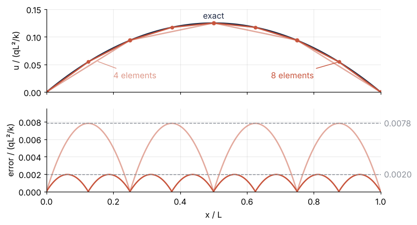
Four elements leave a gap of 0.0078, eight 0.0020, sixteen 0.00049: a factor of 4.00 per halving, and the arches touch zero at every node, so a convergence check at the nodes alone would show nothing. The slope error is h/2, so the heat flux into the blocks comes out as 0.375 against the exact 0.5 with four elements and 0.4375 with eight. It halves with h instead of quartering. The quantity you report decides how fine the mesh must be.
See it in code
The scikit-fem library does the assembly from the weak form, written once for any mesh. Here is the same bar, with four and eight elements:
Show code
from skfem import Basis, ElementLineP1, MeshLine, asm, condense, solve
from skfem.models.poisson import laplace, unit_load

for n_el, U_hand in ((4, U4), (8, U8)):
    mesh = MeshLine(np.linspace(0, L, n_el + 1))
    basis = Basis(mesh, ElementLineP1())
    A = asm(laplace, basis)                        # the integral of u'v' for every pair of hats
    b = asm(unit_load, basis)                      # the integral of v, q = 1, for every hat
    held = condense(A, b, D=mesh.boundary_nodes())  # drop the rows and columns of the end nodes
    u_fem = solve(*held)                           # solves, then puts the held zeros back in
    A_inner = held[0]
    if n_el == 4:
        print(f"stiffness matrix without the end nodes:\n{A_inner.toarray()}")
    print(f"{n_el} elements: U = {np.round(u_fem[1:-1], 5)}")
    print(f"  largest difference from the hand-built U: {np.max(np.abs(u_fem - U_hand)):.0e}")
stiffness matrix without the end nodes:
[[ 8. -4.  0.]
 [-4.  8. -4.]
 [ 0. -4.  8.]]
4 elements: U = [0.09375 0.125   0.09375]
  largest difference from the hand-built U: 1e-17
8 elements: U = [0.05469 0.09375 0.11719 0.125   0.11719 0.09375 0.05469]
  largest difference from the hand-built U: 1e-17
The matrix scikit-fem prints is the hand-built one, rows of 8 and −4, and its nodal values agree with the hand-built ones to rounding, for four elements and for eight. laplace is the left side of the weak form with k = 1, unit_load the right side with q = 1, and condense removes the two held end nodes, as the slicing did above. What the library adds is generality: the element matrices come from numerical integration over a reference element, so the same three lines run on a triangle mesh in two dimensions, which is where scikit-fem from the ground up takes them.
Where it shows up
The heated bar is the simplest case of a pattern that runs through engineering and physics: a quantity spreads by a flux proportional to its gradient, inside a shape too awkward for a formula.
- Stress in structures. Linear elasticity is the vector version of the bar, with displacement for temperature and Young's modulus for conductivity. The words "stiffness matrix" and "load vector" come from here: Boeing engineers in the 1950s computed aircraft wing panels as assemblies of small elastic elements.
- Heat in housings. An electronics enclosure or an engine part obeys \(-\nabla\cdot(k\nabla T) = q\), with k jumping where an aluminum wall meets an air gap. Each element carries its own k, which is the same freedom the bar had with unequal element lengths.
- Groundwater under a dam. Darcy flow, \(-\nabla\cdot(K\nabla h) = 0\) for the hydraulic head, gives the seepage under a foundation and the uplift pressure on its base. findiff.PDE with mixed boundary conditions: seepage under a dam solves it on a grid.
- Electrostatics. The potential around electrodes obeys \(-\nabla\cdot(\varepsilon\nabla\phi) = \rho\), and the field and capacitance of electrodes of arbitrary shape come from its finite element solution. Poisson's equation with scipy.sparse: two plates in a grounded box does the box-shaped case on a grid.
- Bone mechanics. Finite element models of a femur or a vertebra are built from CT scans, one element per voxel, each with a stiffness that follows from the bone density the scan measured. The model predicts the load at which the bone will fracture.
In every case the number that matters is a gradient (stress, heat flux, seepage velocity, field strength), the quantity whose error on the bar fell only in proportion to h.
Further reading
- scikit-fem documentation, for
MeshLine,Basis, and the forms inskfem.models.poisson. - Larson and Bengzon, The Finite Element Method: Theory, Implementation, and Applications (Springer, 2013), whose first chapters treat this one-dimensional problem with code.
- Strang and Fix, An Analysis of the Finite Element Method (1973), for the error estimates.
- Related tutorials on this site: scikit-fem from the ground up: the sag of a membrane under pressure; Finite differences: the heat equation as a matrix, and why the time step has a limit; Finite volumes: why a conservation law is solved by bookkeeping the fluxes; Solve a linear system with NumPy: the currents in a resistor network.
- Download the notebook. It was executed with the library versions in the header.