The lattice Boltzmann method in NumPy: vortex shedding behind a cylinder

The problem: the vortex shedding frequency behind a cylinder

Put a long cylinder across a uniform stream at Reynolds number \(\mathrm{Re} = UD/\nu = 100\) and the wake does not stay symmetric. Vortices peel off one side, then the other, and drift downstream as the Kármán vortex street. The cylinder feels a sideways force that swings back and forth, the lift, measured by the lift coefficient \(C_L = F_y / (\tfrac12 \rho U^2 D)\). The frequency \(f\) of that swing, made dimensionless, is the Strouhal number \(\mathrm{St} = fD/U\), and Williamson's experiments give 0.164 at Re = 100.

We will compute it with the lattice Boltzmann method, which never discretizes the Navier-Stokes equations. Each cell of a square lattice holds nine numbers, the amounts of fluid moving in nine directions. Every time step they move to the neighboring cell they point at and relax toward a local equilibrium that conserves mass and momentum. On scales large compared with a cell, density and velocity then obey the Navier-Stokes equations, with a viscosity set by the relaxation time. There is no Poisson equation for the pressure to solve at every step, as in the usual incompressible solvers, and the price is that the fluid is slightly compressible: it has a sound speed, and it behaves like an incompressible fluid only while the flow is much slower than that. The Navier-Stokes equations and the Reynolds number are assumed from a fluids course.

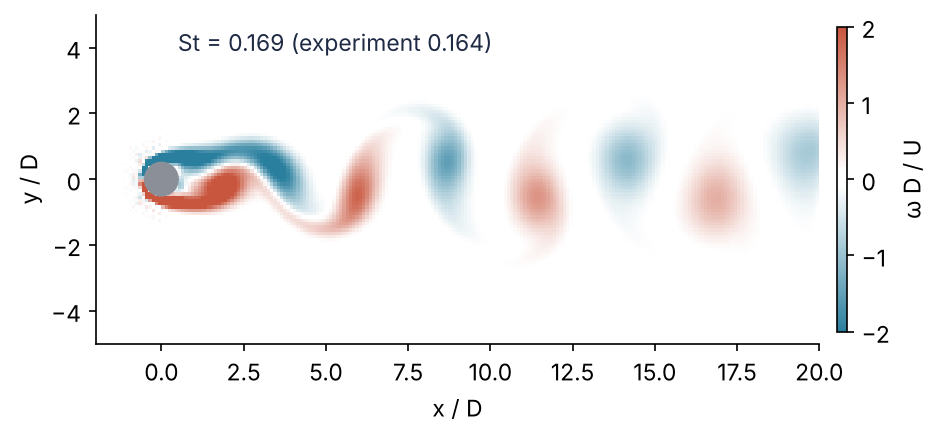
Vorticity behind a cylinder at Re = 100 computed with the lattice Boltzmann method, x and y in cylinder diameters. Red and teal vortices of opposite sign alternate downstream; the Strouhal number 0.169 from the lift is written next to the experimental 0.164.

This is the vorticity after 10,000 steps of the solver you are about to write, with the Strouhal number Step 5 measures.

Setup

Everything runs in lattice units: the cell size is 1 and the time step is 1. Only the Reynolds number has to match the physical flow, so the inflow velocity \(U\) is a free choice, and 0.1 is well below the lattice sound speed of Step 1.

import numpy as np
import matplotlib.pyplot as plt
from matplotlib.colors import LinearSegmentedColormap

NX, NY = 300, 100   # cells along and across the stream
D = 10              # cylinder diameter in cells
U = 0.1             # inflow velocity, lattice units
RE = 100

plt.rcParams.update({
    "figure.figsize": (7.5, 2.8), "figure.dpi": 110,
    "axes.spines.top": False, "axes.spines.right": False,
    "axes.grid": True, "grid.alpha": 0.25,
    "font.size": 11, "lines.linewidth": 1.8,
})
INK, ACCENT, SECOND, MUTED = "#1f2a44", "#c8553d", "#2a7f9e", "#8a8f98"

print(f"grid {NX} x {NY}, D = {D} cells, U = {U}, Re = {RE}")

grid 300 x 100, D = 10 cells, U = 0.1, Re = 100

Step 1: Set up the D2Q9 lattice and its equilibrium distribution

The lattice is called D2Q9: two dimensions, nine velocities \(\mathbf c_i\). One is zero, four point to the neighbors along the axes, four to the diagonal neighbors. Each cell holds nine numbers \(f_i\), the amount of fluid moving with velocity \(\mathbf c_i\). They are also called distributions; I will say populations. Density and momentum are sums over them, \(\rho = \sum_i f_i\) and \(\rho\mathbf u = \sum_i f_i \mathbf c_i\). In the code they share one array f of shape (9, ny, nx): direction first, then \(y\) as the row and \(x\) as the column. The weights \(w_i\) are 4/9 for the rest population, 1/9 along the axes, and 1/36 on the diagonals, the choice that makes the lattice look isotropic up to the moments the Navier-Stokes equations need.

The equilibrium the populations relax toward is

\[f_i^\mathrm{eq} = w_i \rho \left(1 + 3\,\mathbf c_i\cdot\mathbf u + \tfrac92 (\mathbf c_i\cdot\mathbf u)^2 - \tfrac32 u^2\right),\]

an expansion of the Maxwell-Boltzmann distribution for small \(u\), whose coefficients are \(1/c_s^2\), \(1/(2c_s^4)\), and \(1/(2c_s^2)\) with the sound speed \(c_s = 1/\sqrt3\). opp holds the index of the opposite direction, for Step 3. equilibrium broadcasts with None, as in the vectorization tutorial.

c = np.array([[0, 0], [1, 0], [0, 1], [-1, 0], [0, -1],
              [1, 1], [-1, 1], [-1, -1], [1, -1]])       # (c_x, c_y)
w = np.array([4/9] + [1/9] * 4 + [1/36] * 4)
opp = np.array([0, 3, 4, 1, 2, 7, 8, 5, 6])

def moments(f):
    rho = f.sum(axis=0)
    ux = (f[1] + f[5] + f[8] - f[3] - f[6] - f[7]) / rho
    uy = (f[2] + f[5] + f[6] - f[4] - f[7] - f[8]) / rho
    return rho, ux, uy

def equilibrium(rho, ux, uy):
    cu = c[:, 0, None, None] * ux + c[:, 1, None, None] * uy
    return w[:, None, None] * rho * (1 + 3 * cu + 4.5 * cu**2 - 1.5 * (ux**2 + uy**2))

print(f"sum w = {w.sum():.4f}   sum w cx^2 = {w @ c[:, 0]**2:.4f}   sum w cx cy = {w @ (c[:, 0] * c[:, 1]):.4f}")
print("c[opp] == -c for all nine:", np.all(c[opp] == -c))
rho, ux, uy = moments(equilibrium(np.full((1, 1), 1.02), np.full((1, 1), 0.10), np.full((1, 1), 0.03)))
print(f"moments of f_eq: rho = {rho[0, 0]:.6f}, ux = {ux[0, 0]:.6f}, uy = {uy[0, 0]:.6f}")

sum w = 1.0000   sum w cx^2 = 0.3333   sum w cx cy = 0.0000
c[opp] == -c for all nine: True
moments of f_eq: rho = 1.020000, ux = 0.100000, uy = 0.030000

The weights add up to one, the second moment is \(c_s^2 = 1/3\), and the mixed one vanishes. The equilibrium built for \(\rho = 1.02\) and \(\mathbf u = (0.10, 0.03)\) gives back exactly those numbers. That is what makes the method conserve mass and momentum: pushing \(f\) toward \(f^\mathrm{eq}\) changes neither \(\rho\) nor \(\mathbf u\).

Step 2: Stream with np.roll, relax toward equilibrium, and set the viscosity by τ

A time step has two halves. Streaming moves each population one cell along its velocity, one np.roll per direction by \(c_{iy}\) rows and \(c_{ix}\) columns; the wrap-around makes the box periodic in both directions. Top and bottom stay periodic; in \(x\) the inflow and outflow of Step 3 overwrite what wraps around. Collision, in the form called BGK, relaxes every population toward its equilibrium by a fraction \(1/\tau\):

\[f_i \leftarrow f_i + \frac{f_i^\mathrm{eq} - f_i}{\tau}.\]

A loop over the nine directions is faster here than the broadcast equilibrium, because it builds no nine-layer temporaries. The viscosity this produces is \(\nu = c_s^2(\tau - \tfrac12)\), a result of a multiscale expansion called Chapman-Enskog that the books in Further reading derive. Here we check it. A velocity \(u_x = 0.01\sin(ky)\) that points along \(x\) and varies only in \(y\) reduces the Navier-Stokes equations to the diffusion equation \(\partial_t u_x = \nu\,\partial_y^2 u_x\), so the sine keeps its shape and its amplitude decays as \(e^{-\nu k^2 t}\).

def stream(f):
    for i in range(9):
        f[i] = np.roll(f[i], (c[i, 1], c[i, 0]), axis=(0, 1))
    return f

def collide(f, tau):
    rho, ux, uy = moments(f)
    usq = 1.5 * (ux**2 + uy**2)
    for i in range(9):
        cu = 3 * (c[i, 0] * ux + c[i, 1] * uy)
        f[i] += (w[i] * rho * (1 + cu + 0.5 * cu**2 - usq) - f[i]) / tau
    return f

tau = 0.53
nu = (tau - 0.5) / 3
k = 2 * np.pi / 32
y = np.arange(32)[:, None] * np.ones((1, 4))           # 32 rows in y by 4 columns in x, periodic
f = equilibrium(np.ones((32, 4)), 0.01 * np.sin(k * y), np.zeros((32, 4)))
mass0 = f.sum()
amplitude = []
for step in range(1000):
    f = stream(collide(f, tau))
    amplitude.append(2 * np.mean(moments(f)[1] * np.sin(k * y)))   # projection onto the sine
rate = -np.polyfit(np.arange(1, 1001), np.log(amplitude), 1)[0]
print(f"measured decay rate / (nu k^2) = {rate / (nu * k**2):.4f}")
print(f"relative mass drift            = {abs(f.sum() - mass0) / mass0:.1e}")

measured decay rate / (nu k^2) = 1.0032
relative mass drift            = 1.1e-13

The decay rate is within 0.3 % of \(\nu k^2\), and the mass is conserved to rounding. Turned around, the formula sets \(\tau\) from the problem:

nu = U * D / RE
tau = 3 * nu + 0.5
print(f"nu = {nu:.3f}   tau = {tau:.3f}   Ma = U / c_s = {U * np.sqrt(3):.3f}")

nu = 0.010   tau = 0.530   Ma = U / c_s = 0.173

Two limits follow. \(\tau\) must stay above one half, or the viscosity turns negative; 0.530 is 0.03 above it. \(U\) must stay well below \(c_s\), because the equilibrium is an expansion in the Mach number \(u/c_s\) whose density error grows as \(\mathrm{Ma}^2\), here 0.03. Both come back as pitfalls.

Step 3: Put a cylinder in the stream with bounce-back, inflow, and outflow

The cylinder is the set of cells whose centers lie within \(D/2\) of the point \((99.5, 49.5)\). The half-integer center makes the staircase mirror-symmetric and exactly ten cells across. Its wall works by bounce-back: a population that streams into a solid cell is sent back the way it came. What arrived moving east (index 1) leaves moving west (index 3), so f[opp[i]] takes the value of f[i], and the no-slip wall sits about halfway between the last fluid cell and the first solid one.

The inflow sets column 0 to the equilibrium of \(\rho = 1\), \(\mathbf u = (U, 0)\) at every step. The outflow copies the populations of the last column from the column before it, but only the three that move left (\(i\) = 3, 6, 7): after streaming they hold what wrapped around from the inlet.

The symmetric wake at Re = 100 is unstable, but a symmetric simulation has no disturbance to grow, so initial_f adds one: a transverse velocity bump of \(0.1U\), a Gaussian of width \(D/2\) one diameter behind the cylinder. The cylinder cells start at rest, for the reason Step 4 gives.

def cylinder_mask(ny):
    y, x = np.mgrid[0:ny, 0:NX]
    return (x - 99.5)**2 + (y - (ny / 2 - 0.5))**2 < (D / 2)**2

def initial_f(u_in, ny):
    y, x = np.mgrid[0:ny, 0:NX]
    ux = np.full((ny, NX), u_in)
    uy = 0.1 * u_in * np.exp(-((x - 99.5 - D)**2 + (y - (ny / 2 - 0.5))**2) / (2 * (D / 2)**2))
    solid = cylinder_mask(ny)
    ux[solid] = uy[solid] = 0.0
    return equilibrium(np.ones((ny, NX)), ux, uy)

def apply_boundaries(f, solid, f_in):
    f[:, solid] = f[:, solid][opp]                    # bounce-back
    f[:, :, 0] = f_in                                 # inflow
    f[[3, 6, 7], :, -1] = f[[3, 6, 7], :, -2]         # outflow: only the unknown populations
    return f

solid = cylinder_mask(NY)
print(f"solid cells {solid.sum()}, mirror-symmetric: {np.array_equal(solid, solid[::-1])}, "
      f"width {solid.any(axis=0).sum()} cells, blockage D/H = {D / NY:.2f}")

solid cells 80, mirror-symmetric: True, width 10 cells, blockage D/H = 0.10

The cylinder is a staircase of 80 cells. With periodic top and bottom, the flow sees a column of cylinders \(H\) = 100 cells apart, a blockage \(D/H\) of 0.10 that Pitfall 3 doubles.

Step 4: Measure the lift by momentum exchange and run 10,000 steps

Right after streaming, every population that has just crossed from the fluid into the cylinder sits in a solid cell. Bounce-back sends each one back reversed, so its momentum changes from \(\mathbf c_i f_i\) to \(-\mathbf c_i f_i\), and the fluid hands the cylinder \(2\,\mathbf c_i f_i\). The sum over all of them is the force per time step,

\[F_y = 2 \sum_{\text{solid}} \sum_i c_{iy} f_i ,\]

taken after streaming and before bounce-back. For simplicity the code sums over all solid cells, including populations that never left the cylinder. They add nothing while the solid holds fluid at rest, where opposite populations are equal and cancel. That is why the cylinder cells start at rest: with the kick's transverse velocity inside, their \(y\) momentum would flip sign at every bounce-back and add a lift that alternates every step, larger than the shedding.

def run(u_in, re, ny, steps):
    tau = 3 * u_in * D / re + 0.5
    solid = cylinder_mask(ny)
    f = initial_f(u_in, ny)
    f_in = equilibrium(np.ones((ny, 1)), np.full((ny, 1), u_in), np.zeros((ny, 1)))[:, :, 0]
    lift = np.zeros(steps)
    blowup = None
    with np.errstate(over="ignore", invalid="ignore"):   # the pitfalls blow up on purpose
        for t in range(steps):
            f_solid = f[:, solid]
            f = collide(f, tau)
            f[:, solid] = f_solid                           # solid cells do not collide
            f = stream(f)
            lift[t] = 2 * (c[:, 1] @ f[:, solid].sum(axis=1))
            f = apply_boundaries(f, solid, f_in)
            if t % 100 == 0 and not np.isfinite(f).all():
                blowup, lift = t, lift[:t]
                break
        rho, ux, uy = moments(f)
        return lift / (0.5 * u_in**2 * D), ux, uy, rho, blowup

CL, ux, uy, rho, _ = run(U, RE, NY, 10_000)
print(f"C_L over the last 1000 steps: {CL[-1000:].min():+.3f} to {CL[-1000:].max():+.3f}")
print(f"max |rho - 1| = {np.abs(rho - 1).max():.3f}")

C_L over the last 1000 steps: -0.356 to +0.347
max |rho - 1| = 0.021

The lift swings between −0.356 and +0.347, nearly symmetric about zero, and the density varies by 2 %. That is the slight compressibility the method pays for having no pressure equation.

Step 5: Measure the Strouhal number from the lift

Count time in convective units \(tU/D\), the time the stream takes to pass one diameter; 10,000 steps are 100 of them. Leave out the first half, where the oscillation is still growing from the kick, find the upward zero crossings of \(C_L\) by linear interpolation between steps, and average the periods:

def strouhal(CL, u_in, start=5000):
    i = start + np.nonzero((CL[start:-1] < 0) & (CL[start + 1:] >= 0))[0]
    crossings = i + CL[i] / (CL[i] - CL[i + 1])          # fractional step of each zero
    T = np.diff(crossings).mean()
    return D / (u_in * T), T, len(crossings) - 1

St, T, n_periods = strouhal(CL, U)
print(f"{n_periods} periods, T = {T:.1f} steps = {T * U / D:.2f} D/U,  St = {St:.4f}")
D_cm, nu_water = 0.01, 1.0e-6                               # m, m^2/s
U_cm = RE * nu_water / D_cm
print(f"1 cm cylinder in water: U = {100 * U_cm:.1f} cm/s, f = St U / D = {St * U_cm / D_cm:.3f} Hz")

fig, ax = plt.subplots(figsize=(7.5, 2.6))
t_conv = np.arange(len(CL)) * U / D
ax.plot(t_conv, CL, color=ACCENT, lw=1.2)
ax.axvline(50, color=MUTED, ls="--", lw=1)
ax.text(51, 0.42, "measured from here", color=MUTED)
ax.text(78, 0.42, f"St = {St:.3f}", color=ACCENT)
ax.set(xlabel="$t\\,U/D$", ylabel="$C_L$", xlim=(0, 100), ylim=(-0.5, 0.55))
plt.show()

8 periods, T = 592.9 steps = 5.93 D/U,  St = 0.1687
1 cm cylinder in water: U = 1.0 cm/s, f = St U / D = 0.169 Hz

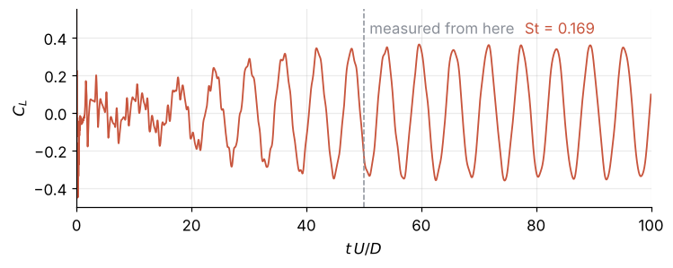
Lift coefficient against time in units of D/U. After a jagged start the oscillation grows and settles by about t = 45 D/U to an amplitude of about 0.35; St = 0.169 is measured from the zero crossings after the dashed line at 50 D/U.

The jagged first 20 \(D/U\) come from the impulsive start, a stream switched on at full speed around a cylinder at rest. Then the lift grows out of the kick, settles by about \(t = 45\,D/U\), and from then on repeats every 5.93 \(D/U\). St = 0.169 is 3 % above Williamson's 0.164, and the blockage of 0.10 is one cause, as Pitfall 3 shows at 0.20. The coarse cylinder is not: twice the cells across \(D\), at eight times the work, moves St slightly up, not down. For a physical cylinder 1 cm across in water, Re = 100 means a stream of 1 cm/s, and the cylinder sheds at 0.169 Hz, one vortex pair every 6 s.

Step 6: Draw the vortex street

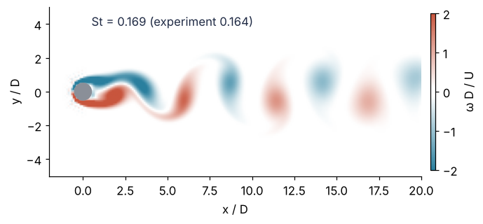
The vorticity \(\omega = \partial u_y/\partial x - \partial u_x/\partial y\) comes from np.gradient on the final field, scaled to \(\omega D/U\). The colormap runs from SECOND (clockwise, negative) through white to ACCENT (counterclockwise, positive) and is clipped at ±2, so the street sets the scale and not the thin boundary layer on the cylinder. Values with \(|\omega D/U|\) below 0.1 are white as well, which hides a grid-scale speckle next to the staircase.

The same field gives the speed of the street. On the centerline \(u_y\) swings up and down once per vortex pair, so its upward zero crossings lie one same-sign vortex spacing apart; they are counted from \(x\) = 120, two diameters behind the center, where the vortices have rolled up.

omega = (np.gradient(uy, axis=1) - np.gradient(ux, axis=0)) * D / U
omega[solid] = np.nan
cmap = LinearSegmentedColormap.from_list(                 # white for |omega D/U| < 0.1
    "street", [(0, SECOND), (0.475, "white"), (0.525, "white"), (1, ACCENT)])

x0, y0 = 99.5, NY / 2 - 0.5                               # cylinder center
crop = slice(80, NX)                                      # from 2 D ahead of the cylinder
extent = [(80 - 0.5 - x0) / D, (NX - 0.5 - x0) / D, (-0.5 - y0) / D, (NY - 0.5 - y0) / D]
fig, ax = plt.subplots(figsize=(7.5, 3.3))
im = ax.imshow(omega[:, crop], origin="lower", extent=extent, cmap=cmap, vmin=-2, vmax=2)
ax.add_patch(plt.Circle((0, 0), 0.5, color=MUTED))
ax.text(0.5, 3.9, f"St = {St:.3f} (experiment 0.164)", color=INK)
ax.set(xlabel="x / D", ylabel="y / D")
ax.grid(False)
fig.colorbar(im, ax=ax, label="ω D / U", shrink=0.8, pad=0.02, aspect=30)
plt.show()

u_mid = 0.5 * (uy[49] + uy[50])                          # transverse velocity on the centerline
i = 120 + np.nonzero((u_mid[120:-1] < 0) & (u_mid[121:] >= 0))[0]
x_cross = i + u_mid[i] / (u_mid[i] - u_mid[i + 1])
spacing = np.diff(x_cross).mean() / D
print(f"spacing of same-sign vortices {spacing:.2f} D, vortex speed {spacing / (T * U / D):.2f} U")

Vorticity behind a cylinder at Re = 100 computed with the lattice Boltzmann method, x and y in cylinder diameters. Red and teal vortices of opposite sign alternate downstream; the Strouhal number 0.169 from the lift is written next to the experimental 0.164.

spacing of same-sign vortices 5.40 D, vortex speed 0.91 U

Vortices of alternating sign leave the upper and lower side of the cylinder and line up in two staggered rows. Two vortices of the same sign are 5.40 \(D\) apart, one period of shedding, so they travel at 0.91 \(U\), a little slower than the stream that carries them.

Pitfalls

A lattice velocity that is too large. It is tempting to raise \(U\), because fewer steps then cover the same \(tU/D\). The equilibrium is an expansion in \(u/c_s\), though, and the density error grows as the square of the Mach number:

for u_in in [0.2, 0.3]:
    _, _, _, rho_p, blowup = run(u_in, RE, NY, 2000)
    result = f"non-finite by step {blowup}" if blowup else f"max |rho - 1| = {np.abs(rho_p - 1).max():.3f}"
    print(f"U = {u_in}  (Ma = {u_in * np.sqrt(3):.2f}): {result}")

U = 0.2  (Ma = 0.35): max |rho - 1| = 0.078
U = 0.3  (Ma = 0.52): non-finite by step 700

At \(U\) = 0.2 the density varies by 7.8 %, nearly four times the 2.1 % of the main run, for twice the Mach number. At 0.3 the run blows up within 700 steps. There is no sharp threshold: keep \(U\) at 0.1 or below and check that max \(|\rho - 1|\) stays at a few percent.

τ too close to one half. Ask for Re = 3000 on the same grid and the run dies:

_, _, _, _, blowup = run(U, 3000, NY, 2000)
print(f"Re = 3000: tau = {3 * U * D / 3000 + 0.5:.3f}, non-finite by step {blowup}")

Re = 3000: tau = 0.501, non-finite by step 1100

Since \(\tau - \tfrac12 = 3UD/\mathrm{Re}\), a higher Re, a lower \(U\) to fix the Mach number, or a smaller \(D\) to save time all push \(\tau\) toward one half. By \(\nu = c_s^2(\tau - \tfrac12)\) that is a vanishing viscosity, and BGK has almost no damping left for the shortest waves on the grid, the same kind of stability limit as the Courant condition in the leapfrog tutorial. The fix is more cells across \(D\), and the three knobs trade against each other. A flow at Re = 3000 is no longer two-dimensional in reality anyway.

Neighbors too close. Halve the height of the box and the periodic images of the cylinder stand \(5D\) apart:

St_50 = strouhal(run(U, RE, 50, 10_000)[0], U)[0]
print(f"H = 5 D (blockage 0.20): St = {St_50:.4f}, {100 * (St_50 / St - 1):+.0f} % against H = 10 D")

H = 5 D (blockage 0.20): St = 0.1930, +14 % against H = 10 D

The images, like channel walls, squeeze the flow past the cylinder and speed it up, and the vortices shed faster. St comes out at 0.193, 14 % above the run with \(H = 10D\) and 18 % above the experiment. Keep \(H\) at \(10D\) or more and state the blockage with the result. A confined channel is a different flow and needs confined reference data.

Variations

Porous medium. Replace the cylinder by a random set of solid disks, make the box periodic in \(x\) as well, and drive the flow with a body force instead of an inflow. The mean velocity against the force gives the permeability, the quantity Darcy's law uses in the seepage tutorial.
MRT collision. Relax each moment of the populations at its own rate instead of all at \(1/\tau\). This stays stable much closer to \(\tau = \tfrac12\) and is the usual cure for the second pitfall.
Three dimensions. D3Q19 has nineteen velocities and its own weights; streaming, collision, and bounce-back stay as they are.
A steady wake. At Re = 40 the cylinder keeps two attached vortices behind it and sheds nothing. Shedding sets in near Re = 47, and sweeping Re across it shows the lift amplitude grow from zero.

Cheat sheet

tau = 3 * U * D / Re + 0.5                                # nu = U D / Re; need tau > 1/2 and U <= 0.1
rho = f.sum(0); ux = (c[:, 0, None, None] * f).sum(0) / rho   # uy likewise with c[:, 1]
cu = c[:, 0, None, None] * ux + c[:, 1, None, None] * uy  # c_i . u, shape (9, ny, nx)
f += (w[:, None, None] * rho * (1 + 3*cu + 4.5*cu**2 - 1.5*(ux**2 + uy**2)) - f) / tau   # BGK; not in solid cells
f[i] = np.roll(f[i], (c[i, 1], c[i, 0]), axis=(0, 1))     # stream, for each i: rows by c_y, columns by c_x
Fy = 2 * (c[:, 1] @ f[:, solid].sum(axis=1))              # lift: after streaming, before bounce-back
f[:, solid] = f[:, solid][opp]                            # bounce-back
f[:, :, 0] = f_in                                         # inflow: equilibrium at (U, 0)
f[[3, 6, 7], :, -1] = f[[3, 6, 7], :, -2]                 # outflow: copy the left-movers
St = D / (U * T)                                          # T in steps; f = St U / D in hertz