Perturbation theory with SymPy: the Duffing oscillator's frequency shift

The problem: a stiffer spring swings faster

A hardening spring, a MEMS beam driven past its linear range, and a string plucked so hard that its tension rises with the stretch all obey, to lowest order, the Duffing equation

\[\ddot x + x + \varepsilon x^3 = 0, \qquad \varepsilon > 0 .\]

Released from rest at \(x(0) = A\) with \(\varepsilon A^2 = 1\), it has a period of 4.768 instead of the linear \(2\pi = 6.283\): 24 % shorter. The Lindstedt-Poincaré method gives that shift as a series in \(\varepsilon A^2\), and SymPy carries the algebra. The equation is in the method's form: \(m\ddot y + ky + \alpha y^3 = 0\) becomes it with time in units of \(1/\omega_0 = \sqrt{m/k}\) and \(\varepsilon = \alpha/k\). Any \(\ddot x + x + \varepsilon f(x, \dot x) = 0\) goes through the same steps.

The obvious attack, \(x = A\cos t + \varepsilon x_1(t) + \dots\), fails at first order: \(x_1\) contains \(-\tfrac38 A^3 t\sin t\), which grows without bound although the energy is conserved. Lindstedt and Poincaré measure time with the unknown frequency instead, \(\tau = \omega t\) with \(\omega = 1 + \varepsilon\omega_1 + \varepsilon^2\omega_2\), and at each order choose \(\omega_k\) so that the forcing at the oscillator's own frequency vanishes. By hand, two orders take pages of trigonometric identities. With SymPy, whose basics are in SymPy from the ground up, they take five steps and end in

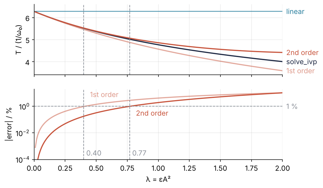
\[\omega = 1 + \frac38\,\varepsilon A^2 - \frac{21}{256}\,\varepsilon^2 A^4 .\]

Top: period of the Duffing oscillator against εA² from 0 to 2: solve_ivp, the first-order and the second-order Lindstedt-Poincaré formulas, and the linear period 2π. Bottom: relative error of each formula in percent, log scale. First order stays within 1 % up to εA² = 0.40, second order up to 0.77.

The top panel sets the period \(2\pi/\omega\) of each truncation against solve_ivp, the bottom panel shows the error. One correction stays within 1 % up to \(\varepsilon A^2 = 0.40\), two corrections up to 0.77. At \(\varepsilon A^2 = 2\) both are off by about 10 %, for the reason in Pitfall 3.

Setup

import numpy as np
import sympy as sp
import matplotlib.pyplot as plt
from scipy.integrate import solve_ivp

plt.rcParams.update({
    "figure.figsize": (7, 4.4), "figure.dpi": 110,
    "axes.spines.top": False, "axes.spines.right": False,
    "axes.grid": True, "grid.alpha": 0.25,
    "font.size": 11, "lines.linewidth": 1.8,
})
INK, ACCENT, SECOND, MUTED = "#1f2a44", "#c8553d", "#2a7f9e", "#8a8f98"

eps, A = sp.symbols("epsilon A", positive=True)
t, tau = sp.symbols("t tau", real=True)     # t: original time, tau: stretched time

print(f"SymPy {sp.__version__}")

SymPy 1.14.0

Step 1: Watch naive perturbation theory fail

Insert \(x = A\cos t + \varepsilon x_1(t)\) into the Duffing equation and keep the terms proportional to \(\varepsilon\). The zeroth order cancels, and what is left is \(\ddot x_1 + x_1 = -A^3\cos^3 t\). sp.Function("x1") creates an undefined function, so that x1(t) is an unknown that diff and dsolve can handle. sp.dsolve solves the equation: it takes the equation and the unknown function, the ics dictionary fixes \(x_1(0) = 0\) and \(\dot x_1(0) = 0\) so that \(x(0) = A\) stays exact, and .rhs takes the right-hand side of the equation it returns. The raw solution hides the interesting term in a mixture of \(\cos^5 t\) and multiple angles, so the cell splits it. On an expanded expression, .coeff(t) returns the factor that multiplies \(t\):

x1 = sp.Function("x1")
naive = sp.Eq(x1(t).diff(t, 2) + x1(t), -A**3 * sp.cos(t)**3)
x1_naive = sp.dsolve(naive, x1(t), ics={x1(0): 0, x1(t).diff(t).subs(t, 0): 0}).rhs

secular = sp.expand(x1_naive).coeff(t) * t
print("growing:", secular)
print("bounded:", sp.simplify(sp.expand(x1_naive) - secular))

growing: -3*A**3*t*sin(t)/8
bounded: A**3*(cos(t)**3 - cos(t))/8

The first line is the failure. \(\cos^3 t\) contains \(\tfrac34\cos t\), a force at the oscillator's own frequency, and an oscillator driven at resonance answers with an amplitude that grows linearly in time. After \(t \sim 1/(\varepsilon A^2)\) the correction is as large as the solution it corrects. A term that grows with \(t\) instead of oscillating is called secular, a name from celestial mechanics, and removing it is the whole method.

Expand a cosine whose frequency is a little off, and the same term appears:

print(sp.series(A * sp.cos((1 + eps * 3 * A**2 / 8) * t), eps, 0, 2))

A*cos(t) - 3*A**3*epsilon*t*sin(t)/8 + O(epsilon**2)

The secular term is a frequency shift written as a power series, and no finite number of terms of it stays right for long. So put the shift into the time variable.

Step 2: Stretch time and sort the equation by powers of ε

With \(\tau = \omega t\) every time derivative picks up a factor \(\omega\), and the equation becomes \(\omega^2 x'' + x + \varepsilon x^3 = 0\), the prime meaning \(d/d\tau\). Into it go two expansions, one for the solution and one for the frequency, with \(\omega_1\) and \(\omega_2\) unknown numbers for now:

x2 = sp.Function("x2")
w1, w2 = sp.symbols("omega1 omega2")

x = A * sp.cos(tau) + eps * x1(tau) + eps**2 * x2(tau)
w = 1 + eps * w1 + eps**2 * w2
eq = sp.expand(w**2 * x.diff(tau, 2) + x + eps * x**3)
orders = [eq.coeff(eps, k) for k in range(3)]

print("order 0:", orders[0])
print("order 1:", orders[1])

order 0: 0
order 1: A**3*cos(tau)**3 - 2*A*omega1*cos(tau) + x1(tau) + Derivative(x1(tau), (tau, 2))

coeff(eps, k) is the tool of Step 1 with a power as second argument: it picks the coefficient of \(\varepsilon^k\), and for \(k = 0\) the terms that contain no \(\varepsilon\) at all. series is not needed, because after expand the expression is a polynomial in \(\varepsilon\) and its coefficients can be read off directly.

Order zero is 0, because \(A\cos\tau\) solves the linear oscillator. Order one is the equation for \(x_1\), with \(A^3\cos^3\tau\) as before and one new term, \(-2A\omega_1\cos\tau\). That term is the handle on the resonance.

Step 3: Remove the resonant term at first order

Move everything except \(x_1'' + x_1\) to the right-hand side and call it the forcing, \(R_1 = 2A\omega_1\cos\tau - A^3\cos^3\tau\). Its \(\cos\tau\) and \(\sin\tau\) components drive \(x_1\) at its natural frequency, and either one produces a secular term, so both must vanish. That requirement is called the solvability condition: the condition under which the equation at order \(k\) has a bounded periodic solution.

By hand you would write \(\cos^3\tau = (3\cos\tau + \cos 3\tau)/4\) and read off the coefficient of \(\cos\tau\). At first order that works. At second order the forcing holds products such as \(\cos^2\tau\cos 3\tau\), and SymPy's simplifiers do not turn powers into harmonics on their own (Pitfall 2). The Fourier coefficient does not care about the form: \(\frac1\pi\int_0^{2\pi} R\cos\tau\,d\tau\) is the \(\cos\tau\) component of \(R\) however it is written, and integrate computes it.

def resonant(R, harmonic=sp.cos):
    return sp.factor(sp.integrate(R * harmonic(tau), (tau, 0, 2 * sp.pi)) / sp.pi)

R1 = x1(tau).diff(tau, 2) + x1(tau) - orders[1]
print("cos part:", resonant(R1))
print("sin part:", resonant(R1, sp.sin))

w1_val = sp.solve(resonant(R1), w1)[0]
eq1 = sp.Eq(x1(tau).diff(tau, 2) + x1(tau), R1.subs(w1, w1_val))
x1_sol = sp.dsolve(eq1, x1(tau), ics={x1(0): 0, x1(tau).diff(tau).subs(tau, 0): 0}).rhs
print("omega1 =", w1_val)
print("x1     =", x1_sol)

cos part: -A*(3*A**2 - 8*omega1)/4
sin part: 0
omega1 = 3*A**2/8
x1     = -A**3*cos(tau)/32 + A**3*cos(3*tau)/32

The sine part is zero because \(R_1\) is even in \(\tau\); for the Van der Pol oscillator in Variations it is not. Setting the cosine part to zero gives \(\omega_1 = 3A^2/8\), the coefficient the identity by hand gives and the one Step 1's series showed. The initial conditions are zero again, so \(x(0) = A\) holds at every order. \(x_1\) has \(\tau\) only inside cosines: no secular term. At \(\varepsilon A^2 = 0.1\) this first-order value raises the frequency by 3.75 %. The true rise is 3.67 %, from the period of 6.0607 that Step 5 measures there.

Step 4: Go to second order

The order-\(\varepsilon^2\) equation contains \(x_1\) and \(\omega_1\), which are now known. Substitute both and call .doit(): subs puts the expression for \(x_1\) inside the Derivative objects of the equation but does not differentiate it, and doit does. Then come the same projection and solve. The forcing is again even in \(\tau\), so its sine part is zero and the cell checks only the cosine. \(\omega_2\) does not need \(x_2\), so the code does not compute it.

known = {x1(tau): x1_sol, w1: w1_val}
R2 = x2(tau).diff(tau, 2) + x2(tau) - orders[2].subs(known).doit()
print("cos part:", resonant(R2))

w2_val = sp.solve(resonant(R2), w2)[0]
omega = 1 + eps * w1_val + eps**2 * w2_val
print("omega2 =", w2_val)
print("omega  =", omega)

cos part: A*(21*A**4 + 256*omega2)/128
omega2 = -21*A**4/256
omega  = -21*A**4*epsilon**2/256 + 3*A**2*epsilon/8 + 1

The second correction is negative. The first order overestimates the frequency, so the period it predicts is too short, and Step 5 measures by how much.

Step 5: Check the period against solve_ivp

The formula has two parameters, and the check needs only one. Substitute \(x = y/\sqrt\varepsilon\) into the Duffing equation and \(\varepsilon\) drops out: \(\ddot y + y + y^3 = 0\), released at \(y(0) = \sqrt\varepsilon\,A\). Every pair \((\varepsilon, A)\) with the same \(\lambda = \varepsilon A^2\) is the same motion, rescaled, so the numerical side sets \(\varepsilon = 1\) and \(A = \sqrt\lambda\) and loses nothing. Small in the expansion means small \(\lambda\), not small \(\varepsilon\).

lambdify turns the two truncations of \(2\pi/\omega\) into NumPy functions of \(\lambda\). The measured period uses the upward-crossing event of solve_ivp from the ground up, with tight tolerances. The period never exceeds \(2\pi\) for a hardening spring, so a window of \(4\pi\) always holds two upward crossings. Two hundred solver calls cover \(\lambda\) from 0.01 to 2:

lam = sp.symbols("lambda", positive=True)
T_first = sp.lambdify(lam, (2 * sp.pi / (1 + eps * w1_val)).subs(A, sp.sqrt(lam / eps)))
T_second = sp.lambdify(lam, (2 * sp.pi / omega).subs(A, sp.sqrt(lam / eps)))

def duffing(t, y):
    return [y[1], -y[0] - y[0]**3]

def upward(t, y):
    return y[0]
upward.direction = 1

def period(lam):
    s = solve_ivp(duffing, (0, 4 * np.pi), [np.sqrt(lam), 0.0],
                  events=upward, rtol=1e-10, atol=1e-12)
    c = s.t_events[0]
    return c[1] - c[0]

lams = np.arange(1, 201) / 100
T_num = np.array([period(l) for l in lams])
err1 = 100 * (T_first(lams) - T_num) / T_num
err2 = 100 * (T_second(lams) - T_num) / T_num

def last_within(err, limit):
    return lams[np.argmax(np.abs(err) > limit) - 1]   # last λ before the first miss

print("  λ    T (solve_ivp)   1st order   2nd order")
for l in [0.1, 0.3, 0.5, 1.0, 2.0]:
    i = np.argmin(np.abs(lams - l))
    print(f"{l:4.1f}   {T_num[i]:10.4f}   {err1[i]:+8.3f} %  {err2[i]:+8.4f} %")
for limit in [1, 0.1]:
    print(f"within {limit:g} %: first order up to λ = {last_within(err1, limit):.2f}, "
          f"second order up to λ = {last_within(err2, limit):.2f}")

  λ    T (solve_ivp)   1st order   2nd order
 0.1       6.0607     -0.075 %   +0.0036 %
 0.3       5.6809     -0.583 %   +0.0815 %
 0.5       5.3667     -1.408 %   +0.3247 %
 1.0       4.7680     -4.162 %   +1.9186 %
 2.0       4.0043    -10.337 %  +10.3547 %
within 1 %: first order up to λ = 0.40, second order up to λ = 0.77
within 0.1 %: first order up to λ = 0.11, second order up to λ = 0.32

At \(\lambda = 1\) the second order is off by 1.92 % where the first was off by 4.16 %, and the range of a 1 % formula grows from \(\lambda = 0.40\) to 0.77, nearly double. The signs confirm Step 4: the first order is always too short, the second too long. At \(\lambda = 0.3\) the first-order period is already 0.58 % off, which for a high-Q MEMS resonator is many linewidths. Plotted against the measured period:

fig, (ax_T, ax_e) = plt.subplots(2, 1, sharex=True, height_ratios=[1, 1])
ax_T.axhline(2 * np.pi, color=SECOND, lw=1)
ax_T.plot(lams, T_num, color=INK)
ax_T.plot(lams, T_first(lams), color=ACCENT, alpha=0.5)
ax_T.plot(lams, T_second(lams), color=ACCENT)
for y, label, color, a in [(2 * np.pi, "linear", SECOND, 1), (T_num[-1], "solve_ivp", INK, 1),
                           (T_first(2.0), "1st order", ACCENT, 0.6), (T_second(2.0), "2nd order", ACCENT, 1)]:
    ax_T.text(2.03, y, label, color=color, alpha=a, va="center")
ax_T.set(ylabel="T / (1/ω₀)", ylim=(3.4, 6.6))

ax_e.semilogy(lams, np.abs(err1), color=ACCENT, alpha=0.5)
ax_e.semilogy(lams, np.abs(err2), color=ACCENT)
ax_e.text(0.45, 5, "1st order", color=ACCENT, alpha=0.6)
ax_e.text(0.82, 0.2, "2nd order", color=ACCENT)
ax_e.axhline(1, color=MUTED, lw=1, ls="--")
ax_e.text(2.03, 1, "1 %", color=MUTED, va="center")
for err in [err1, err2]:
    l1 = last_within(err, 1)
    for ax in (ax_T, ax_e):
        ax.axvline(l1, color=MUTED, lw=1, ls="--")
    ax_e.text(l1 + 0.02, 2e-4, f"{l1:.2f}", color=MUTED)
ax_e.set(xlabel="λ = εA²", ylabel="|error| / %", xlim=(0, 2), ylim=(1e-4, 20))
plt.show()

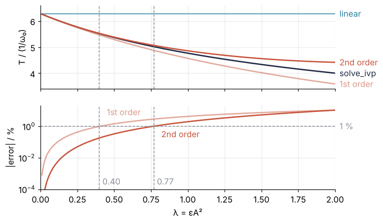
Top: period of the Duffing oscillator against εA² from 0 to 2: solve_ivp, the first-order and the second-order Lindstedt-Poincaré formulas, and the linear period 2π. Bottom: relative error of each formula in percent, log scale. First order stays within 1 % up to εA² = 0.40, second order up to 0.77.

The two error curves meet near \(\lambda = 2\), which is where Pitfall 3 picks up.

Pitfalls

A means something else in your textbook. You get \(-15/256\) for the second-order coefficient where a book has \(-21/256\), or the other way around. Both are right, for different \(A\). Here \(A\) is the initial displacement, and that gives \(-21/256\). Other books take \(A\) as the amplitude of the \(\cos\tau\) harmonic and demand that \(x_1\) have no \(\cos\tau\) part. Then \(x_1 = A^3\cos 3\tau/32\), the motion starts at \(x(0) = A + \varepsilon A^3/32\), and the coefficient is \(-15/256\). Say which one you use, and in the code it is the ics you hand to dsolve.

Waiting for a simplifier to show the harmonics. You expect SymPy to reduce \(\cos^3\tau\) the way you would by hand, and it does not:

from sympy.simplify.fu import TR8

c3 = sp.cos(tau)**3
print("trigsimp:", sp.trigsimp(c3))
print("fu:      ", sp.fu(c3))
print("TR8:     ", TR8(c3))

trigsimp: cos(tau)**3
fu:       cos(tau)**3
TR8:      3*cos(tau)/4 + cos(3*tau)/4

A simplifier aims for a short expression and promises no particular form, and \(\cos^3\tau\) is already short. For the resonant term you do not need the harmonics at all: the projection of Step 3 finds it in any form. When you want them on screen, TR8 from sympy.simplify.fu applies the product-to-sum rules and shows them.

More orders are not more range. At \(\lambda = 2\) the first order is off by \(-10.3\) % and the second by \(+10.4\) %: the added term overshoots by as much as the first one fell short. The frequency is a power series in \(\lambda\), and a power series converges only inside its radius of convergence, the distance from zero to the nearest point where the function breaks down. Here that point is \(\lambda = -1\). A softening spring (\(\varepsilon < 0\)) released at \(|\varepsilon| A^2 = 1\) starts exactly on top of its potential hill at \(x = 1/\sqrt{|\varepsilon|}\) and never comes back, so its period is infinite, and a series in \(\lambda\) cannot reach past that distance on either side of zero. The radius is 1, and \(\lambda = 2\) lies outside it. Trust the expansion for \(\lambda\) well below 1, and above that integrate, as in Step 5.

Variations

The pendulum. Replace \(\varepsilon x^3\) by \(-\varepsilon x^3/6 + \varepsilon^2 x^5/120\), the series of \(\sin x\) after its linear term. Two orders give \(\omega = 1 - \theta_0^2/16 + \theta_0^4/3072\), whose inverse is the \(T/T_0 = 1 + \theta_0^2/16 + 11\theta_0^4/3072\) that SymPy from the ground up derives from the period integral. Here \(\varepsilon\) only counts orders and is set to 1 at the end, with \(A = \theta_0\), which is how the method handles a problem with no small coefficient. Without the \(x^5\) term the second order comes out wrong.
A softening spring. Take \(\varepsilon < 0\), as for a MEMS beam softened by an electrostatic field. Declare eps real instead of positive: Steps 2 to 4 never use its sign and return the same \(\omega\), now with \(\lambda < 0\), so the period lengthens. In Step 5, duffing gets \(+y^3\), period starts at np.sqrt(-lam) and needs a window longer than \(4\pi\), and the sweep stays above \(\lambda = -1\), the hilltop of Pitfall 3.
The Van der Pol oscillator. \(\ddot x + x = \varepsilon(1 - x^2)\dot x\), with \(\omega\,x'\) in place of \(\dot x\) inside the forcing. Now the sine part is not zero, and the two conditions give \(\omega_1 = 0\) and \(A = 2\): the amplitude of the limit cycle, the closed orbit every solution settles onto. solve_ivp from the ground up integrates the same equation in its stiff pitfall.

Cheat sheet

x = A*sp.cos(tau) + eps*x1(tau) + eps**2*x2(tau)          # x1, x2 = sp.Function("x1"), sp.Function("x2")
w = 1 + eps*w1 + eps**2*w2                                 # tau = w*t, t in units of 1/omega0
orders = [sp.expand(w**2*x.diff(tau, 2) + x + eps*x**3).coeff(eps, k) for k in range(3)]  # your eps*f here
R1 = x1(tau).diff(tau, 2) + x1(tau) - orders[1]            # forcing of x1'' + x1
w1_val = sp.solve(sp.integrate(R1*sp.cos(tau), (tau, 0, 2*sp.pi)), w1)[0]  # sin part must vanish too
x1_sol = sp.dsolve(sp.Eq(x1(tau).diff(tau, 2) + x1(tau), R1.subs(w1, w1_val)), x1(tau),
                   ics={x1(0): 0, x1(tau).diff(tau).subs(tau, 0): 0}).rhs   # x(0) = A at every order
R2 = x2(tau).diff(tau, 2) + x2(tau) - orders[2].subs({x1(tau): x1_sol, w1: w1_val}).doit()
w2_val = sp.solve(sp.integrate(R2*sp.cos(tau), (tau, 0, 2*sp.pi)), w2)[0]  # lam = sp.Symbol("lambda") = eps*A**2:
T = sp.lambdify(lam, (2*sp.pi/(1 + eps*w1_val + eps**2*w2_val)).subs(A, sp.sqrt(lam/eps)))